In this Part of the Thesis we develop techniques that relate to robotics. Geometric Algebra has found relatively widespread use in the analysis of robots. GA simplifies the intersection of geometric shapes, often used in forward and inverse kinematics, and GA provides a neat framework for the manipulation of Lie algebras and groups, again often useful in forward and inverse kinematics as well as in control problems. Here we specifically look at the embedding of screw theory into Geometric Algebra and how this embedding can be used for dynamics and multi-body kinematics.
We may always depend on it that algebra, which cannot be translated into good English and sound common sense, is bad algebra.William Kingdon Clifford
Screw Theory and Geometric Algebra (GA) are mathematical frameworks that have found wide use in the analysis of robotic mechanisms. Here we consider an embedding of screw theoretic wrenches and twists into the motor bivectors of two common GAs, the Plane-based (also known as Projective) and Conformal Geometric Algebras. We start with statics, considering the representations of forces and moments and how the products of GA map to the products of Screw Theory. Moving on from statics we construct an inertia tensor equivalent based on the concept of the principal screws of inertia and show how to transform this inertia tensor between frames of reference. We then look at the problem of geometrically constrained dynamics in two different ways, first via the familiar concept of virtual work, and secondly via a novel idea of multivector pinning between frames. Finally we consider the problem of integrating screw motions directly in the motor bivector space, describing kinematic equations for several alternative se(3) Lie algebra to Lie group mappings. Our goal in this chapter is to kill two birds with one stone: explicitly work through how Screw Theory embeds into commonly used GAs and use Screw Theoretic ideas to show the similarity between the various approaches to statics and dynamics in GA. Along the way we will focus heavily on the geometry driving the problems we encounter, with the hope that this will shed light both on both GA and Screw Theory.
Screw theory was originally developed by Sir Robert Stawell Ball (1840-1913) and described in his seminal text `A Treatise on the Theory of Screws'
Ball [1900]. Screw Theory has found wide adoption in the study of 3D mechanisms as it allows a simple, unified treatment of both the rotational and translational motion of rigid bodies. The Screw Theory literature draws on multiple sources of mathematics but Lie theory and Projective Geometry feature heavily. Modern Screw Theory appears in several different forms and is referred to by various different names by different authors. From the `spatial vector algebra' of Roy Featherstone
Featherstone [2008,
2010] to the `Linear Line Complexes' of Helmutt Pottmann
Pottmann and Wallner [2001] the diversity of terminology reflects the diversity of fields in which Screw Theory has found applications and mathematical foundations. This chapter is an attempt to articulate a particularly elegant embedding of Screw Theory into the coordinate free language of Geometric Algebra (GA) and how this novel embedding might allow us to push the boundaries of Screw Theory in new directions.
Conformal Geometric Algebra (CGA) is a real Clifford algebra with signature

. It is very popular for its embedding of conformal transformations (and so also the Euclidean transformations) as well as its blade representations of many geometric primitives. CGA is especially well suited for robotics as the direct circle and sphere intersections appear in many forward and inverse kinematic problems while the motions involved are typically Euclidean
Hadfield and Wieser [2020];
Hadfield et al. [2020]. CGA was first suggested by Hestenes
Hestenes et al. [1985] and indeed the same author made the first steps in uniting it with Screw Theory
Hestenes and Fasse [2002];
Hestenes [2010]. CGA has since been applied to a huge variety of problems, for more information about this algebra the reader is directed to the excellent book of Dorst, Fontijne and Mann
Dorst et al. [2007].
While CGA has been a very successful idea it is by no means the most computationally efficient way to embed rigid body dynamics into GA. In many applications a practitioner is willing to lose some of the expressiveness and mathematical niceties of CGA to gain an algebra with fewer elements that nonetheless does what they desire, and crucially, does it computationally
faster. The Plane-based (or Projective) Geometric Algebra (PGA) aims to strike a balance between efficiency and expressiveness. With a signature of

it contains the so called `flat' elements of CGA, flat points, direction bivectors, lines, planes and the rigid body rotors, but loses point-pairs, circles, spheres, dilation and inversion rotors as first class citizens of the algebra. The use of the degenerate metric also necessitates the use of an alternate dual map rather than a simple multiplication by the pseudoscalar, in practice this dualisation operation can be implemented by the right complement extended over the canonical basis vectors by linearity. For more information on PGA the reader is directed towards the 2019 SIGGRAPH course by Gunn and De Keninck
Gunn and De Keninck [2019a,
b] and Leo Dorst's `A Guided Tour to the Plane-Based Geometric Algebra PGA'
Dorst [2020].
While this chapter is ostensibly about dynamics we will first cover force representations and static equilibrium to make sure we are developing sensible mathematics before we put things in motion.
For a rigid body to be in static equilibrium certain conditions have to be met. Specifically, there can be no net moment (torque) and no net force acting on it.
We will now do a quick survey of the different force representations, and in doing so, think about what an effective force representation requires.
In many approaches to mechanics, forces are formalised as a simple 3D vector aligned with the direction of the force and a magnitude equal to the intensity of the force. In order to calculate the resultant force on a rigid body acted upon by many incident forces we take the vector sum of the force vectors acting on the body. To represent a moment in the same formalism we use a 3D vector parallel to the axis of the moment with magnitude equal to its intensity and with the convention that a positive turning force acts counter-clockwise about this axis. To calculate the moment of a force about a specific point on the body we need to combine the incident force with its incident position. If we label the force vector

, its incident point

and the point about which we aim to calculate the moment as

then we can calculate the moment

with the cross product:
The 3D vector representation is efficient and easy to understand, however it does not encode all the information that exists in our idea of a force. Specifically, it does not inherently include any localisation information about the force. When we want to calculate the moment due to the force about a specific point we need to include the additional information of a point on the line of action of the force. Therefore to be able to use this representation effectively we
actually require two 3D vectors, one the 3D force vector
and one determining a point
through which the force acts. We can stack these two 3D vectors on top of each other to make a 6D vector which we will call

:
This object
now contains all the information required to use the force in applications. It is however
not unique. We could choose multiple values of
all of which lie on the line and they would all give different 6D representations of the force while still fundamentally behaving the same way physically. To solve this problem we need to instead use a representation of the force that is unique. If we change our representation to:
then we get such a formulation, as all points on the line of action of the force will have the same result for

. This 6D representation is known as the Plücker coordinates of the line
Pottmann and Wallner [2001].
In contrast to a force, a moment is not localised to a specific point or line in the world, in the terminology of physics and engineering this type of non-localised vector is known as a free vector. While respecting their non-localised nature we would like to be able to put the 3D moments in the same 6D box as forces to be able to keep the representations consistent and maybe provide some meaningful operations on them. When putting our 3D moment vector into the 6D box we are left with several different options. One option would be to put the moment vector in the top 3 positions of the 6D vector, such that they align with the component of the force, or maybe we should put them in the lower 3 to make them align with the part of the force representation.
Initially, which choice to make seems non-obvious. To help us gain some insight we consider the problem of two anti-parallel co-planar forces of equal magnitude acting on a rigid body. First, label the forces themselves:
In this situation, as the forces are in opposite directions and of equal magnitude, the total resultant force on the body is

. But what about the total moment

of the forces about a point
on the body?
As the cross product is distributive we can expand this out and rearrange it giving:
This is an interesting result. The moment is independent of the position
on the rigid body that we have taken moments about and is equal simply to the sum of the second half of our 6D force representation. This concept of two anti-parallel forces giving rise to a pure moment is the basis of the term
couple or
force couple from mechanical engineering. If we were to write an external moment in the form:
We could exploit the linear independence of the top and bottom of the 6D vector to state our static equilibrium condition as:
This is a neat result and gives us hope that continuing down the route of 6D representations will lead us to other interesting things.
In fact continuing down this route leads us to the concept of constructing an algebra over these 6D objects, known as the algebra of screws and more generally into the territory of the field known as Screw Theory. The basic element of such a `screw algebra' is a 6D vector made up of the 6D representation of a force line and the 6D representation of a moment with axis parallel to that force line. Or, more formally,
where

are 3D vectors and

is a scalar. Chasles' theorem states that we can, in fact, decompose any 6D vector into this form. In the language of Screw Theory pure forces and pure moments are both special cases of the more general
wrenches, which is the name for the 6d representation of a screw representing a combination of force and moment. Screw Theory goes on to define a couple of useful products between screws. The first product is the `reciprocal scalar product' of screws which, for two screws

and

of the form
gives a scalar:
where here the

operator is the standard inner product between vectors.
The second product we will consider is the screw cross product, for screws
and
the screw cross product gives:
where

and

are computed with the standard 3D cross product. The result of the cross product of two screws is itself another screw.
Representations of wrenches in CGA and PGA
So far we have dealt entirely with the realm of forces and moments and their representation in 6D screw theory where they are known as wrenches.
We have not yet touched on the main topic of the thesis, Geometric Algebra (GA). Our goal in this section will be to describe a direct mapping from our 6D screw theory representation to two of the most commonly used GAs, namely CGA and PGA.
In the previous section on the screw representation we saw how we could describe a force as a directed line with a magnitude using a 6D vector. Let us now consider how we might go about representing a force line in CGA. As before consider a force line

expressed as 6D Plücker coordinates:
We could represent this same force in CGA as the outer product of two conformal points and infinity:
where we use the notation
up
to represent the mapping of a 3DGA point to a conformal point, ie.
 up
up
.
The object

has a magnitude equal to the intensity of the force:
Now consider the dual form of this CGA line:
 |
(63) |
This looks very similar to the 6D Plücker representation, in fact if we consider it closely we can see that it is the same. First, look at the term in front,

. This is the 3D dual to a 3D vector, giving a bivector, specifically the Euclidean bivector orthogonal to
. Now consider the second half of the formula:

.

is the 3D dual to a Euclidean bivector, ie. a vector equal to
, just like the lower 3 slots of the 6D screw representation. As

is a Euclidean vector this makes
the form of a CGA `direction bivector'. An important thing to note here is that the front and back part of this formula are linearly independent, just like in the 6D screw representation, ie.
Again as with the 6D representation we can consider two anti-parallel forces and extract the representation of a force couple or moment. Setting

and

in the above leaves us with:
which we could re-write as:
where
is a 3D vector.
As previously mentioned this is in the form of a CGA `direction bivector'. These bivectors have the interesting property of being invariant to the action of translation rotors, effectively making them free vectors in the physics sense. Physically, two anti-parallel forces create a force couple, a pure moment, and so we will take objects of the form

to be representations of moments in our scheme. This seems apt as, physically, a pure moment is often thought of as a free vector.
Let us now look at the products of GA. Consider two objects of the form:
The geometric product between them gives:
In general this is a mixed grade object, if we expand out the geometric product between vectors it will give us some insight what these grades signify geometrically:
Now collect the terms by grade:
where
From this grade-based breakdown it is quite easy to see how the different parts of the result relate to the various products of Screw Theory. First, the reciprocal product of screws, which in our 6D representation produced a scalar. In our CGA formulation this scalar maps to the coefficient of

in the result of our geometric product, ie.
As
and
are in fact bivectors we can also write this in terms of the outer product:
Next we consider the bivector part of the geometric product result, alongside the cross product of screws:
If we rewrite the GA formula here:
then equating terms gives:
and
The form of the standard vector cross product in 3D GA is, for vectors
and
, given by:
This means we can represent the cross product of screws via the negative of the bivector part of the geometric product result. In fact, we can write the bivector part of the result in terms of the `commutator product' of geometric algebra which is also, unsurprisingly perhaps, written using the `

' notation.
For readers well versed in Screw Theory, Clifford/Geometric Algebra and Lie Theory this is a well known result. The commutator product equips the motor bivectors with a Lie bracket just as the cross product equips the screws with one. In fact we can go further into the idea of the motor bivector as an element of

and note that the grade 0 element of the geometric product, equal to the GA dot product between the bivectors, is proportional to the Killing form
Minguzzi [2013],

, of the Lie algebra ie.

.
In PGA a line is computed as the intersection of two planes. As by default in PGA we are in a so called `inner product null space' or IPNS we perform the intersection of these two planes by the outer product. We first break this down component-wise for the intersection of two planes:
which we can now re-write this in terms that look more familiar:
In this form the line looks very similar to the CGA representation of the line. The line squares to a scalar, there is a section that is a Euclidean bivector and a section that is a null bivector. In fact the only thing that we have changed is the form of the null element. In CGA we typically use the null element

constructed from the sum of two orthogonal basis vectors, one squaring to

and one to

. Here in PGA the null element

is itself a basis vector. For our 6D force line representation we therefore have exactly the same mapping as we did in CGA:
and so moments appear as:
We would also expect the various products of Screw Theory to still appear as the various grades of the result of a geometric product between two elements of this algebra. Indeed they are the same as the CGA results, but of course replacing
with

which is now the pseudo-scalar of the algebra.
Different authors have taken different approaches when considering the form of forces in conformal and projective geometric algebra. In Lasenby, Lasenby and Doran's `Rigid Body Dynamics and Conformal Geometric Algebra'
Lasenby et al. [2011] the conformal force representation is taken to be of the form
where
is the normal Euclidean 3D force vector and

is a scalar multiplier. This force formulation is then wedged with
and combined with their equation (1.42) to define the equations of motion. When wedged with
this force takes the form:
this is in the form of a direction bivector.
This paper further goes on to specify in equation (1.50) that the form of the moment bivector that a force of this type generates about a point is:
We can break this up into its constituent parts as follows:
This moment formulation is then wedged with
and combined with their equation (1.42) to define the equations of motion. We now consider, as they do in their equation (1.55), the form of the moment wedged with
:
Now take the dual of this quantity with respect to 5D pseudoscalar:
This is the bivector form of a CGA line in the direction of the 3D vector
and passing through the point

.
`Rigid Body Dynamics and Conformal Geometric Algebra' Lasenby et al. [2011] therefore uses a mixture of 1-vectors and bivectors to represent forces but in the end their static equilibrium conditions are in the form of bivectors and trivectors, indeed they are left with something very similar to our formulation in section 6.2.2. The main difference in fact is related to which of the two orthogonal elements of the wrench formulation we take to be a moment and which to be a line. Lasenby et al. effectively choose the
 part to be a force and here we choose the dual line section to be the force.
In fact conceptually our approach here of having lines as forces is the same as Charles Gunn's approach in his paper `On the Homogeneous Model of Euclidean Geometry' Gunn [2011a] and his PhD Thesis Gunn [2011b]. To make this connection more explicit consider the form of a PGA `ideal line', used to represent moments in Gunn's formulation:
where

. The properties of this object are that it squares to 0, ie. it is null but that the magnitude and direction of the 3D vector
are the magnitude and axis of the moment. This is identical to the

formulation for bivector moments that we described in section
6.2.2.
As discussed in Anthony Lasenby's `Rigid Body Dynamics in a Constant
Curvature Space and the ‘1D-up’ Approach
to Conformal Geometric Algebra' Lasenby [2011], both `On the Homogeneous Model of Euclidean Geometry' Gunn [2011a] and `Rigid Body Dynamics and Conformal Geometric Algebra' Lasenby et al. [2011] use the same form for rotors and generalised instantaneous velocities, known in the Screw Theory literature as twists.
Before looking at dynamics in detail, we will define the notation used and state various definitions.
We will consider a world that contains a single rigid body. A frame is rigidly attached to the rigid body and the body moves through space such that a time varying rotor  will transform an arbitrary fixed point
  in the body frame into the corresponding point
  in the world frame:
We will take time derivatives. As
is fixed:
Now substitute in

and

:
A rotor by definition has the property that

.
If we differentiate this constraint with respect to time
which means we can write:
which is twice the anti-commutator of
and

. If
is a 1-vector and as
is a bivector we can write:
If we now label our bivector quantity:
 |
(64) |
it allows us to write:
 |
(65) |
where
represents the commutator product.
Note that in this form with the commutator product no assumptions are made of the grade or other properties of . If we do restrict
to 1-vectors however, this allows us to write:
We can further re-arrange equation (6.3) to get an equation for the relationship between the rotor and its time derivative in terms of this quantity  :
:
 |
(66) |
This quantity
is actually our generalised instantaneous screw velocity, expressed in the world frame. Geometrically it is a screw and we can transform it just like any other screw between frames. We can therefore write

and change equation (
6.5) to:
 |
(67) |
where

is the velocity bivector expressed in the body frame. For reference the reverse of this quantity is:
In the screw theory literature
is known as a `twist' or `velocity screw'.
To take further time derivatives we can just use the chain rule:
 |
(68) |
and we will also calculate the reverse for reference:
In traditional 3D dynamics formulations we specify that the resultant force is the rate of change of linear momentum and the resultant moment is the rate of change of angular momentum. In a screw formulation we can specify that, for a body under the influence of multiple external forces

, the resultant wrench

is the rate of change of screw momentum

with time:
We can, of course, write this whether we are working in the 6D vector space, CGA or PGA.
In 3D dynamics we are used to the idea of converting between linear velocity and linear momentum via multiplication or division by the mass of the rigid body. For a body of mass

and linear velocity

the linear momentum is simply

:
When it comes to angular velocity,

, and angular momentum,

, however we have a more complicated relationship. In fact, for a body centred and axis aligned reference frame, the two are related by a diagonal matrix known as the inertia tensor that we label here as

:
where
can be expressed in the form of

, the second moments of volume:
While it is clear that our screw equivalent of the inertia tensor should also be a linear function that somehow combines the linear and rotational aspects of the above and maps between screw velocity and screw momentum it is not immediately obvious how we should go about constructing such a function. Let us write the matrix version of this linear function for now as
 and the GA version as
  :
:
To solve the problem of determining this function we will construct a little thought experiment. Imagine a rigid body that is initially at rest at the origin but which is then acted on by a wrench  . The velocity of objects attached to the frame of the body are given by:
By differentiating this equation we can calculate the acceleration of objects in the frame:
![$\displaystyle \ddot{X} = \dot{X} \times Q^{-1}[\Psi] + X \times Q^{-1}[\dot{\Psi}]
.$](img929.svg) |
(69) |
In this case the body is initially at rest implying
 allowing us to eliminate the first term and leaving us with:
![$\displaystyle \ddot{X} = X \times Q^{-1}[\dot{\Psi}] = X \times Q^{-1}[W] .$](img931.svg) |
(70) |
We therefore have a direct mapping from the wrench acting on the body to the initial acceleration of objects in the frame and we can now use our physical intuition about the world to guide us to a compatible form of

and hence
.
To calculate the form of this linear function in GA we will first have to define what is known in the GA literature as a reciprocal frame. An important thing to note here is that this is different to the concept in screw theory of a screw and a twist being reciprocal Gallardo-Alvarado [2016] which we will come to later when considering virtual work and power. What we mean by a reciprocal frame here is a set of reciprocal bases  that are matched to the motor bivectors
  such that when the GA inner product is taken between the two matched elements the result is 1 but otherwise 0, ie.:
These reciprocal frame constructs are fairly common in the GA literature and are especially useful for this type of problem.
As is a linear function operating on a motor bivector in CGA it can be written as:
![$\displaystyle Q^{-1}[W] = \sum_i \left[ (S^i\cdot W) \sum_k c_{ik} S_k \right]$](img935.svg) |
(71) |
where

are scalar coefficients,
is the reciprocal frame for the motor bivectors and

are the motor bivectors themselves. We will take
and
as follows:
and will seek to determine

. This formulation is equivalent to a square matrix formulation of
where the coefficients
are the elements in the matrix. What we need to do here is to find out exactly what these
coefficients have to be.
Firstly we will probe the response of the function to the action of a force passing through the centre of mass of the object, which lies at the origin. We can write such a force as a dual line in CGA as:
where in this case
is 0 as we are at the origin, giving:
The mapping that embeds a 3D point
in CGA is given by:
which, after differentiation twice leads to:
As the body is initially stationary,

is zero and so we have for time

:
For the case of a force of magnitude

applied to the centre of mass of a rigid body we would expect all points on the body to accelerate linearly at

in the direction of
, or more formally

for all
. We can encode this expectation by substituting

and
into equation (
6.9):
![$\displaystyle (\ddot{x} \cdot x)n_{\infty}+ \ddot{x} = \left(\frac{1}{2}x^2n_{\infty}+ x + n_0\right) \times Q^{-1}[W]$](img951.svg) |
(72) |
and we can then apply our specific case:
Looking closely at
we can see that

is a Euclidean bivector and, when dotted with each of the reciprocal frame elements in turn it is non zero only for
![$[-e_1I_3,\, -e_2I_3,\, -e_3I_3]$](img955.svg)
in which cases the dot product gives only

, the component of the force in the

direction. In other words we could write:
where

and

. We can combine this with

to give:
Let us now examine the terms on the right hand side of the above equation:
For
![$S_k \in e_n\wedge n_{\infty}, n \in [1,2,3]$](img965.svg)
we have the results that

,

,

.
For
![$S_k \in [e_1I_3,\,\, e_2I_3,\,\, e_3I_3]$](img969.svg)
we have the results that

,
.
Now we can consider the above equation component-wise and extract the required transformation coefficients. Firstly, consider the coefficients of
:
Expand the left side into a sum of elements of the force vector:
Comparing terms we see we have arrived at the following solution:
Now that we have dealt with the
terms we can return to the Euclidean bivectors:
We have just calculated the

terms in the right hand side of this equation and so by substituting these in we get something of the form:
which implies that

. A visual representation of the argument made here can be seen in Figure
6.1.
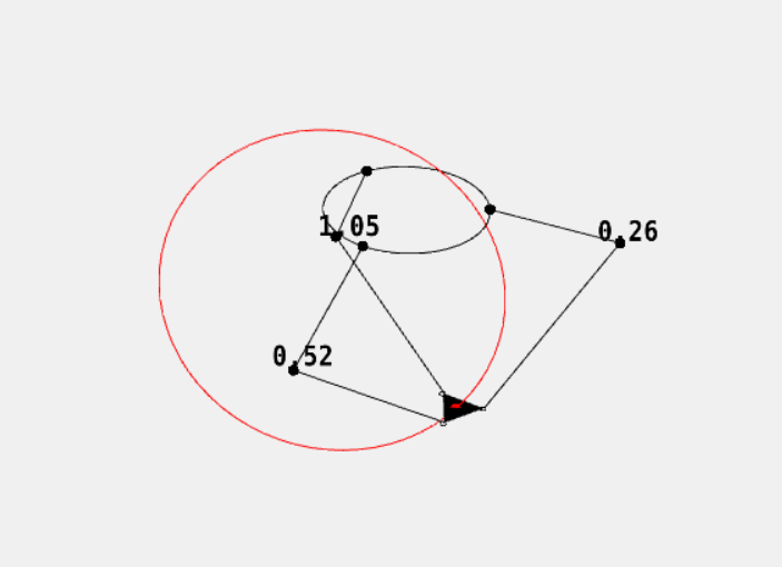
Fig. 6.1:
The multivector field generated by the commutator product of a twist and a field of multivector points can be visualised and provides a visual verification of the action of specific types of twist. Here we are visualising a twist in the form of a `direction bivector' which produces a uniform linear velocity field. This implies that our inertia tensor, or indeed some preprocessing step to the inertia tensor, must map from lines through the origin to direction bivectors, a fact proved in the mathematical content of this section.
|
Fig. 6.2:
As in Figure 6.1 here we are visualising the multivector field generated by the commutator product of a twist and a field of points. Here the twist that is visualised is a line through the origin. The field that is generated is rotational about the line. Again as with the translational field of Figure 6.1 this implies specific constraints on our inertia tensor and shows the inherent reciprocal nature of momentum screws/wrenches and velocity twists in the Screw Theory formulation of dynamics.
|
So far we have dealt with all the translational elements of the transformation, however we have only prescribed 18 of the total 36 (66) degrees of freedom of the problem. To continue calculating the required form of the transformation we will now analyse the effect of a torque applied to the rigid body. Firstly we will again need the general form of the acceleration of a point due to a wrench:
 |
(74) |
We will now apply a moment to the rigid body, again at rest at the origin. From standard 3D kinematics we know that if we have a body rotating about its centre of mass and about an axis  with angular speed
  , ie.
, ie.
 then, provided that the centre of mass has no linear velocity we can calculate the linear velocity of a point on the body as:
and the acceleration of a point as:
where
is the traditional cross product operation. In this thought experiment the body is initially at rest allowing us to remove the
term and leaving us with:
where

is the 3d torque vector. The GA equivalent of the traditional 3d cross product for vectors
and
is

. Which means we can write:
We can represent this same moment in our CGA formulation as the bivector wrench

. Again we look at:
and from this we note that

for
![$S^i \in [-e_nI_3]$](img992.svg)
and that

for
![$i \in [4,5,6]$](img994.svg)
. For this case we can therefore write equation (
6.13) as:
The left hand side of this equation collapses simply to

and we bring
inside the summation again on the right:
We can now use the same results as noted previously to simplify the right hand side of this equation, leading to:
Equating like terms eliminates all the
terms, ie.

for
. This leaves us with:
We can break up the left side of this component-wise:
Now assume that our torque vector is aligned with one of the principal axes of the rigid body, say

, this implies

is only non-zero for

:
Which is true because

.
Noting that

allows us to identify the

parameters:

,

,

.
Of course our choice of as the principal axis to which our torque vector aligns was arbitrary, we could equally have chosen one of the other two principal axes,  and
and  with their respective
  and
and  . As a result of this symmetry we can directly identify our final parameters:
 ,
,
 ,
,
 ,
,
 ,
,
 ,
,
 .
.
Figure 6.2 gives a graphical illustration of why this form of mapping is required for rotations and torques.
The Screw Inertia Tensor
For our 6D vector representation had we not just done the maths of the previous section we might have been tempted to stack the and on top of each other to produce a combined inertia tensor like:
This however would ignore the fundamental conceptual differences in the action of the top 3 and bottom 3 elements of the 6D representation as a wrench vs as a twisting motion generator. Instead, we need to use the coefficients
of the last section to produce a matrix that performs a `flip' in the relative positions of the parts of the vectors while also applying the required scaling along each principal axis. Putting the calculated coefficients in place we can see that the matrix that comes out for
looks like this:
We could also achieve this `flip' effect via a diagonal matrix and a permutation matrix:
 |
(75) |
where

is the

identity matrix.
When writing the inertia tensor in CGA it is convenient to do a little relabelling for ease of reading. The reciprocal frame of the motor bivectors in CGA is as follows:
Which we can break into the two groups:
and so with these we can write the inertia tensor:
and the inverse inertia tensor:
This inertia tensor performs the same kind of `flip' that we saw for the 6D screw representation. Effectively our inertia tensor does the following mapping:
The reciprocal frame construction of the inertia tensor that we have discussed so far works for many algebras but for degenerate metric algebras such as PGA the fact that we have an element squaring to zero means this setup does not work. Instead we need to do something a little different. The degenerate metric approach to reciprocal frames
Gunn [2020] is to consider some blade which we will label

that wedges with a given blade of magnitude

ie

to produce the pseudoscalar with magnitude
ie.

. Clearly, despite us labelling it
, this object is not quite the same as the reciprocal frame, although it allows us to perform the same function of coordinate free coefficient selection producing the magnitude
as the scalar coefficient of the pseudoscalar. Let us now identify this pseudo-reciprocal frame for the PGA bivectors:
Comparing the PGA pseudo-reciprocal frame mapping with that of our CGA-inertia tensor mapping it is immediately clear that they are equivalent up to a minus sign. We will now define a function to perform this PGA mapping and will call it

.
has the following action:
where the syntax

returns the scalar coefficient of

in

. We can extend this operation to combinations of basis elements by linearity so that for

:
As with our CGA reciprocal frame let's now write our PGA pseudo-reciprocal frame in two groups:
This means we can write our PGA inertia tensor as:
and its inverse inertia tensor:
We could also apply the
map first to first `flip' the input and apply a component-wise scaling
to the result:
This
map first formulation is conceptually the same as the screw formulation with a flip permutation matrix as in equation (
6.14).
We can visualise the motor bivectors as a frame of screws attached to the origin. These motor bivectors are a version of the Principal Screws of Inertia, specifically they are the principal screws in a Plücker and Hunt sense as opposed to Ball's original formulation of the principal screws. Effectively what we are doing in the inertia tensor is considering these principal screws as wrenches and analysing the impact of them on the motion of the body.
By considering the bivectors as localised screws we can begin to build intuition about them and their properties. First of all, we will consider how they, and their reciprocal frame, transform under the action of rigid body rotors. The Euclidean bivectors are in the form of a dual line through the origin and are affected by rotors exactly as lines are. The direction type motor bivectors (
 ) are, as we mentioned previously, invariant to translation rotors but are affected by rotation rotors. For the general case of the rigid body rotor the direction bivectors therefore are affected only by the rotational aspect of the rotor. This is in keeping with the view of these bivectors as dual lines at infinity, known in the projective geometry world as `ideal' lines.
The transformation properties of the motor bivectors suggests an inroad on the problem of defining non-axis aligned inertia tensors which often comes up in analysis problems when we wish to transform the frame of a body to be about a known axis of rotation. We can phrase this specific problem as follows. Consider a body with a known, axis aligned, inertia tensor  and a world frame momentum . We can get the velocity of the body by transforming the world frame momentum back to the body frame, applying the inverse inertia tensor, and transforming back:
We will wrap this

operation up as an inertia tensor in its own right and label it

, we can therefore write:
 |
(76) |
The problem of defining non-axis aligned inertia tensors is, given we know

and
, exactly what form does
take?
The form of is:
Based on the fact we can transform screws and their reciprocal frames with rotors as usual, we will guess the form of
to be as follows:
![$\displaystyle Q_W^{-1}(\Psi) = \Omega = \frac{1}{m}\sum_{i=1}^{i=3}\left[ \frac...
...lde{R}))(Rl_i\tilde{R}) + (\Psi \cdot (Rl^i\tilde{R}))(Rt_i\tilde{R}) \right] .$](img1078.svg) |
(77) |
Note this is just the same as

except that we have transformed all of the motor bivectors and reciprocals by
, effectively transforming the frame of principal screws to be centred and aligned with the rigid body but expressed in the world frame. We can check whether our guess is correct as follows. Substitute

:
Noting that

and

we can write:
We can then take the rotor application outside of the summation by factorisation and we have arrived at the required relation of equation (
6.15):
Of course by allowing the movement of the frame of the inertia tensor with the body it will no longer be constant and we therefore might also want the form of the time derivative for potential applications:
 |
(78) |
In this subsection we have analysed the principal screws as CGA objects and our analysis of the translation of the inertia tensor was phrased using the transformation of the reciprocal frame. In reality we could equally have done our analysis from the PGA perspective as well, with our pseudo-reciprocal frame taking the place of the reciprocal frame and so our equivalent transformed inverse inertia tensor would appear as:
Fig. 6.3:
A cuboid is simulated spinning about its 2nd principal axis of inertia while translating linearly. Due to the intermediate axis theorem small instabilities in the rotation build quickly causing rapid flips in orientation. Despite these rapid flips the linear motion of the centre of mass is unaffected. Blue: the path of the centre of mass, Green, Red, Orange: the path of several vertices on the cuboid as it undergoes a flip in orientation.
|
Equipped with forces, moments, momentum, velocities and inertia tensors we are now at a position where we can formulate the equations of motion and simulate them. We will start by considering the dynamics of an unconstrained rigid body moving under the influence of external forces and moments. We can write the state of our rigid body at a time as:
and its first time derivative is:
where

is the momentum bivector at time
expressed in the world frame and

is the resultant external wrench acting on the body expressed in the body frame. From this point on we will drop the
subscript and simply state that all variables are functions of time. From our discussion in the previous section we know that we can further expand
using the inverse inertia tensor
:
Re-writing the time derivative of the state with this equation for
gives:
Unconstrained dynamics, while important, do not allow us to represent all the types of motion that we see in the real world around us. In many practical situations we are faced with the problem of constrained motion. Consider modelling a rigid body that can move dynamically under external forces but is constrained so that one or more points lie on a surface or a situation where a rigid body is constrained such that it can translate but not rotate. These are the types of problem we will attack here.
To impose a constraint on our dynamics model we will use the concept of a reaction wrench. The reaction wrench provides a combined external force and moment that acts on the rigid body in addition to the other external wrenches and, in doing so, forces the body to move in a way that respects the constraints. We will write  as the sum of external wrenches, , plus some reaction wrench, , caused by the constraints. As we already know , all we need to calculate is the value of required to keep the constraints valid.
In traditional constrained dynamics work the concepts of virtual work and virtual power are widespread. In the virtual work/virtual power literature constraints are enforced by imagining several independent virtual reaction forces and moments at the constraint position and ensuring that any velocity of the body produces zero power against these forces/moments. In the screw framework that we have developed, the virtual power,  , produced by a virtual world frame wrench, , when the body moves with a body frame screw velocity is given by:
and is of the form
where
is a virtual scalar power. Differentiating this gives:
We can now substitute in our dynamics equation for

:
Setting the virtual power and rate of change of virtual power to 0 gives us the virtual power condition for our constraint. First:
tells us that the virtual wrench must be parallel to the screw velocity. Setting the rate of change of virtual power to be zero allows us to write:
If
is a static constraint we can specify that

leaving us with:
Which can again be solved for
and hence
.
If we specify the way that varies with time we can add curved surface constraints. Consider a situation in which a rigid body is constrained such that one point always touches a sphere centred at point  . Given the point is always touching the sphere we know that must always be parallel to the line joining and , we would therefore write:
Taking a time derivative of this we see:
As
is driven by the rotor
, ie:
we get:
and so:
We can then directly substitute this into:
and so calculate
. To constrain this same point to a circle we would add an additional planar constraint, ie. the point must lie on the plane in which the circle lies and on the sphere of which the circle is the equator.
Consider a geometric primitive represented by multivector  in the body frame and the same geometric primitive represented by multivector when expressed in the world frame. These two multivectors can be related by the rotor :
or equivalently:
Taking first and second derivatives gives us the expressions:
 |
(79) |
 |
(80) |
The next step is to think about what these expressions mean physically. Essentially we have two `views' of the same object, one in body space and one in world space. For example we can imagine the
is a point attached to our rigid body and
is a point in the world that that point is also attached to. In a sense we are `pinning' the rigid body to
by its extremity
.
Lets consider first the case that both of these `views' of the object are fixed, ie. the position and orientation of cannot change with respect to the coordinate system of the body and the position and orientation of cannot change with respect to the origin. Mathematically we are stating that
 . If we substitute these values into (6.19) for the time derivatives we end up with the following equation:
 |
(81) |
This equation is a constraint on the second time derivative of
that will ensure that
and
do not vary with time. We can go a step further here and substitute our expression for

from equation (
6.7), leading to:
Now if we substitute in

and

:
Simplify and gather, substituting

:
Now separate the terms with
:
As

are bivectors their reverse is just a negation:
 |
(82) |
So far, we have done a lot of algebra but so far appear to be no closer to calculating our reaction wrench. If we calculate an expression for
however, we start to make headway towards a solution:
using

we can also write:
![$\displaystyle = Q^{-1}[\dot{\tilde{R}}\Psi R + \tilde{R}\Psi\dot{R}] + Q^{-1}[W_b]$](img1135.svg) |
(83) |
and so we can now substitute in on the left hand side of equation (
6.21) for
:
Now we separate out the terms with
and take all terms not containing
onto the right side of the equation. We now have something of the form:
![$\displaystyle -\frac{1}{2}Q^{-1}[W_b]U + \frac{1}{2}UQ^{-1}[W_b] =$](img1138.svg)
Some function of

We can rewrite this to use the commutator product:
![$\displaystyle (U\times Q^{-1}[W_b]) =$](img1140.svg) Some function of Some function of |
(84) |
If we now decide to write our total bivector wrench,
, as the sum of external wrenches,
, plus some reaction wrench,
, caused by the constraints:
![$\displaystyle (U\times Q^{-1}[F]) = -(U\times Q^{-1}[S]) +$](img1141.svg)
Some function of

we now have a constraint expression that fixes the reaction wrench
as a function of the state of the system and the forces applied to it.
For a given
 this constraint is linear in and can be solved for so long as we provide a correct basis for the constraint wrench. An important point to make here is that this discussion has been entirely algebra agnostic. This framework works equally well for CGA, PGA or indeed many other geometric algebras, a topic that we will return to later on.
Now that we have identified a means of enforcing constraints via pinned geometric primitives let us have a look at exactly what constraints are imposed by specific choices of this pinned multivector for CGA and PGA.
If we want to pin a specific point in our rigid body to a point in the world we can set an invariant point constraint. In this case
and
are both points and, due to the rotational symmetry of a point our reaction wrench
can only support translational forces and no moments. In this case
has 3 degrees of freedom, corresponding to each of the translational principal screws of inertia. This point constraint can be set in both CGA and PGA.
Consider a bivector

of the form:
where
and

are CGA points. This object is invariant only under the action of rotation rotors about an axis parallel to the line joining
and
. In this case
has 5 degrees of freedom corresponding to 3 translational forces and 2 moments. This point-pair constraint is specific to CGA.
Consider a so called `direction' bivector in CGA of the form:
where

is a 3D vector. This object is invariant under the action of all translation rotors and is invariant to rotation rotors with axis of rotation parallel to
, ie. rotors of the form:
where

is the pseudoscalar of 3D space. In this case
only has 2 degrees of freedom corresponding to two moments with axes perpendicular to d. For a PGA equivalent of this constraint a bivector of the form:
can be used to achieve the same thing.
Consider a so called `flat point' bivector in CGA of the form:
where
is a 3D vector. This object is invariant under the action of all rotation rotors about the point
, but is not invariant to translation. Thus, under the action of the rigid body rotors it behaves like a CGA 1-vector point. For PGA this constraint can again be implemented by a standard PGA point.
A line is invariant to translation along the line and rotation about the line axis. Thus we would expect to be able to support reaction forces orthogonal to the line, and moments with axes orthogonal to the line axis, ie.
has 4 degrees of freedom. In PGA a line is a bivector and is formed by the intersection of two planes, in CGA a line can be represented directly as the wedge of two points and
or dually as given in equation (
6.2). Both the dual and direct CGA form work fine for pinning.
Fig. 6.4:
Left: A physical pendulum moves under the effect of gravity and with a starting linear momentum. It is constrained such that a line, coincident with one end of the pendulum shown in blue, is pinned between the body and world reference frames. The symmetry of the line leads to constrained motion along and about the line.
Right: A spinning cone is affected by gravity but is constrained such that its end point, shown in blue, does not move. Precession and nutation are observable in the movement of the centre of mass, shown in green, and a point on the rim of the cone, shown in red.
|
A circle is invariant to rotation about the axis of the circle only. Thus we would expect to be able to support reaction forces in all directions and all moments other than the one with axis parallel to the circle axis, in other words
has 5 degrees of freedom. In retrospect this should be unsurprising as the dual to a 3-vector CGA circle is an imaginary point-pair bivector, and we have already seen that point-pairs have this same form of invariance.
Fig. 6.5:
A physical pendulum moves under gravity and is constrained such that one end of it, shown in blue, is always in contact with the surface of an object. The green trace shows the midpoint of the pendulum and the red shows the free end. Left: a sphere. Right: a circle.
|
A plane is invariant to translation in plane and rotation about axes parallel to its normal direction. Thus it can support one direction of force and two directions of moments giving 3 degrees of freedom to
. Both CGA and PGA can use planes for pinning.
A sphere is invariant to all rotation about its centre, but not to translation. Thus it acts like a point at the sphere centre and
can support translation reaction forces only giving it 3 degrees of freedom. CGA can represent spheres directly as the outer product of 4 points. In PGA this type of constraint would have to be enforced by pinning a point at the centre of the sphere.
So far in our construction of multivector pinning constraints we have assumed that the objects we are pinning are static in both the world and body frame. When working with constrained dynamics in the real world we often want to pin parts of our rigid body to moving things in the real world, such as a manipulator attached to the moving end-point of a robot, or a flywheel fixed in a moving vehicle. Consider once again equation (
6.19):
In the previous section we enforced static multivector constraints by setting

to zero, rearranging to isolate the
terms and solving the resultant linear equation for
. Now we will relax the static constraint and consider the cases when

are known
time varying multivector functions, ie when

.
First note we can still rearrange to separate terms in :
In fact, if we continue as in our previous analysis by breaking up
as a function of
and extracting
:
and so:
If we substitute
we have eventually got to a position where:
![$\displaystyle (U\times Q^{-1}[F]) =$](img1163.svg)
Some function of

Again this is a linear function in
and so solvable as long as it is of sufficient rank.
What this means practically is that we can set and to follow any desired path we like in their respective spaces and extract the reaction forces and moments acting on the body that are required to keep them pinned to each other.
In the previous two sections we dealt directly with transformations that pin static multivectors or time varying multivector paths directly to each other in space. In many practical situations what we would really like to pin is a linear function of one multivector to another. For example we could pin the outer product of a point in the body frame and a plane in the world frame to 0, effectively forcing them to be coincident without specifying anything about their relative orientation (unlike in the transformed plane invariant case). Mathematically we can express our linear function constraint as
![$A[\,]$](img1165.svg)
and time derivatives as:
Once again we can rearrange:
leading to an equation of the form:
Again this is linear and solvable as before. Figure
6.5 shows the simulation with the Clifford Python library
Hadfield et al. [sent] of two cases in which the linear function is the outer product with one end of a physical pendulum.
Throughout this chapter so far we have represented the derivative of the state of the body on the motor manifold as

. In practice numerical integration schemes which integrate
will undoubtedly accumulate errors and so wander off the motor manifold. Depending on the application this may or may not be a problem
Boyle [2017]. We can, however, nicely side step the problem by directly mapping the velocity screw to a velocity in a suitable se(3) Lie algebra that generates the rotor
. If we label the generator for the current position and orientation in the Lie algebra as

which maps to the current rotor with a function
then we are interested in finding a function
that does the following:
We will refer to this function
as the `kinematic equation' for the given Lie algebra to Lie group mapping and will have a look at its form for a few choices of
.
One commonly used mapping for SE(3) is the exponential mapping:
Conveniently, the kinematic equation for the exponential mapping of the motor bivectors has already been derived in
Candy [2012] and a screw Lie algebra version in
Selig [2004] and appears again (with a corrected typo) at the end of Section 4.5 in
Selig [2005]. The result in
Selig [2004,
2005] is derived via idempotents and nilpotents of the adjoint matrix representation of the se(3) Lie algebra but it is readily translatable into our own notation:
where

.
The exponential se(3) kinematic equation is also the subject of Section 5.3 of Liam Candy's PhD thesis Candy [2012], and while the set up of the problem is certainly correct we were unable to make their equation 5.41 work in our implementations. Suspecting simply a typo somewhere in their derivations of the derivatives we can calculate the derivatives ourselves and check the final result. We start with the following setup, following mostly along the lines of Candy [2012]. Our objective is to calculate
 as a function of and
  or . First, we note that it is possible to write a motor bivector in the form:
 |
(86) |
where
is a rotation bivector and
is a 3DGA vector. We then follow
Candy [2012] choosing to define two quantaties:
where:
We can then write an expression for
as the time derivative of (
6.25):
This is made up of the following components:
where:
If we restrict ourselves to so(3) these equations will produce the same answer as that of the Bortz equation
Bortz [1971] familiar to practitioners from the field of strapdown inertial navigation.
An alternative mapping to the exponential that is simple and potentially useful is the Cayley mapping
Hestenes and Fasse [2002];
Tingelstad and Egeland [2018]. For small rotations and translations the Cayley mapping approximates the exponential however it diverges somewhat as we move further from the origin. Matrix versions of the Cayley map are well known and the kinematic equations for the matrix versions of this map have been studied before in the aeronautics literature
Sinclair [2005]. We have failed to find any previous attempts at the GA version of the kinematic equation however we can reuse much of the logic of the matrix derivation, simply substituting transposes for tildes. Start with the expression for the mapping:
 |
(87) |
Take the time derivative:
Rearrange:
Now we will seek a reformulation of

:
This allows us to write:
and so we are left with:
 |
(88) |
The final mapping that we will consider is the so called `outer exponential' mapping as presented in
Tingelstad and Egeland [2018]. This mapping is defined as taking a Taylor series of the exponential but replacing geometric products with wedge products, for an algebra with maximum grade 5 or below this can be written as:
 |
(89) |
Again we were unable to find a GA kinematic equation for this mapping in the existing literature and so present our own as follows. First we take a time derivative of the outer exponential:
Then, given that in (
6.3) we have defined:
we can therefore write:
Noticing that:
and rewriting our equation for
as:
gives us:
We can now equate grade 0 elements:
and so:
We can also equate grade 2 elements:
This, after some rearrangement, leaves us with the form of the kinematic equation for the outer exponential:
We can write this neatly as:
![$\displaystyle \dot{\Phi } = \frac{1}{2}\sqrt{1-\langle \Phi ^2\rangle } \left[-...
... \langle \Omega_w R \rangle \langle R\rangle _2} { \langle R\rangle } \right] .$](img1216.svg) |
(90) |
In this chapter we have looked at forces, moments, free and constrained dynamics in both CGA and PGA. As well as considering how to apply virtual power as a constraint mechanism in our GA formulations we have constructed a novel technique for constrained dynamics in GA via the concept of multivector pinning. While in this chapter we have only considered two algebras, CGA and PGA, the techniques are expected to work across the board for algebras with easily representable line elements and motor bivectors. Using other higher dimensional algebras such as Cl(4,4)
Du et al. [2017], Cl(8,2)
Easter and Hitzer [2017] or even Cl(9,6)
Breuils et al. [2018] with this technique in the future should allow for easy configurations of exotic constraints such as pinning dynamic objects to the surface of quadrics.
Wealth, beauty and fame are transient. When those are gone, little is left except the need to be useful.Gene Tierney
Screw Theory is a framework for analysing articulated mechanisms and performing statics and dynamics calculations that has found much success in the kinematic analysis of mechanisms. In this chapter we consider the embedding of Screw Theory into another extremely powerful framework for robotics, namely Geometric Algebra (GA). We start by rederiving well known results for the accumulation of twists along kinematic chains within our GA framework before turning our attention to the analysis of kinematic pairs. We derive an elegant representation of kinematic pairs via bilinear functions of basic geometric primitives and use this to describe the most common types of robotic joints. We then address multi-body systems and, using the Delta robot as a case study, we compare the screw theoretic approach to a direct differentiation method for extracting the Jacobians of the system.
Modern manufacturing is increasingly mechanised and automated. The drive for automation has led to a need for advanced modelling capabilities and many modern analysis frameworks have been developed as a result. Perhaps the most successful of these frameworks for the analysis for 3D mechanisms is known as Screw Theory. Screw Theory is, unsurprisingly perhaps, concerned with the study of `screws'. In its modern form Screw Theory was first described by Sir Robert Stawell Ball in his `Treatise on the Theory of Screws'
Ball [1900], however the mathematical roots that underlie this remarkable field come from Projective Geometry
Pottmann and Wallner [2001] and the study of Lie groups and Lie algebras
Selig [2004]. More recent proponents of Screw Theory include Hunt
Hunt [1991], Selig
Selig [2005], Davidson
Davidson and Hunt [2004], Martins
Selig and Martins [2014];
Tischler et al. [2000], Featherstone
Featherstone [2008], Gallardo Alvarado
Gallardo-Alvarado [2016], Pottmann
Pottmann and Wallner [2001], Minguzzi
Minguzzi [2013], Lipkin
Lipkin [2005] and indeed many others.
Alongside the development of Screw Theory, and indeed building on some of the same fundamental mathematics, we have seen the rise of the Clifford/Geometric Algebra (GA) as a robotics modelling framework Aristidou [2010]; Fu et al. [2013]; Hildenbrand et al. [2008,2019]; Kim et al. [2015]; Kleppe and Egeland [2016]; Tichý [2020]; Zamora and Bayro-Corrochano [2004]. With modern computing capabilities, the high level description of geometry that these algebras afford allows researchers elegant, concise and coordinate-free descriptions of physically intricate mechanisms and constraints. Many of the modern applications of GA are in the analysis of conformal Dorst and Valkenburg [2011] and Euclidean motions Gunn [2011b], however there have been only a few attempts to properly embed the tools of modern Screw Theory into GA Hestenes and Fasse [2002]; Tingelstad and Egeland [2018]. This chapter, along with the previous one, is an attempt to lay out the overlap between the two fields with language and ideas familiar to both Screw Theory and GA practitioners.
In this chapter we will, by default, work with Conformal Geometric Alegbra (CGA). CGA adds two more basis vectors,

and

, to the original basis vectors of 3D Euclidean space, giving a complete basis for the 5D space with the following signature:

and

. These extra basis vectors are used to define two null vectors:

and

– note that the

notation was that originally used when Hestenes first introduced this model in
Hestenes et al. [1985]. The mapping from a 3D vector,
, to its corresponding CGA vector,
, is given by:
 |
(91) |
which is often referred to as:
up
. We can invert this mapping quite easily so long as we remember to normalise the CGA point such that

:
where

. There are many excellent expositions on CGA in the literature and so we will refrain from a lengthy introduction of all the features of the algebra in this chapter, instead simply preferring to remind the reader of immediately relevant facts about the framework as we go along. If the reader is looking for a more thorough coverage of CGA we would recommend they turn to the excellent book
Geometric Algebra for Computer Science by Dorst, Fontijne and Mann
Dorst et al. [2007].
One of the important sections of the CGA framework that this chapter will deal with is the set of bivectors that form the generators of rotors that perform Euclidean motion, we will refer to these bivectors as the motor bivectors. The motor bivector basis set contains 6 elements, reflecting the 6 degrees of freedom present in rigid body motion. A common choice for the motor bivector basis in CGA is the following ordered set:
where
represents the 3D pseudo-scalar

. This set would have a corresponding reciprocal frame as follows:
such that

if

and

if

. The full set of motor bivectors is then a linear combination of this motor bivector basis. Introducing 6 scalar parameters
we can write a general motor bivector
as:
An alternative and increasingly popular GA framework to work in is the Plane-based or Projective Geometric Algebra (PGA)
Dorst [2020];
Gunn [2011b]. This algebra has signature Cl(3,0,1), meaning it has 3 basis vectors that square to
, 0 basis vectors that square to
and one null basis vector that squares to
0. It is a subalgebra of CGA that contains only the `flat' elements and the Euclidean rotors
Hrdina et al. [2021];
Lasenby [2011]. Restricting the algebra in this way is useful for certain applications that do not require the round elements of CGA and especially as the reduced dimensionality can produce significant speedups for some numerical packages. PGA also contains the motor bivectors with its null basis vector,
taking the place of
. Due to its degenerate signature PGA cannot use reciprocal frames in the same way as CGA but this restriction can be neatly sidestepped via pseudo-reciprocal frames as described in
Gunn [2020] and explicitly worked through for the motor bivectors in Chapter
6. While PGA is not a direct focus of this specific chapter a sharp eyed reader will note that almost all of the formulae in the Screw Theory framework developed here will work with no, or only minor, modifications in PGA.
Whichever GA you choose, the motor bivectors, when exponentiated, produce rotors that can implement rigid body motions. In general it is possible to split into two commuting bivectors, one a generator of rotational motion about a line in the world and one a generator of translational motion along that line. This combination of rotational and translational motion leads to the identification of the motor bivectors as `screws' and if we were to take the 6 scalar parameters and arrange them in a 6x1 vector we would get the vector space that is the core subject matter of the field of Screw Theory. This chapter is one of a pair which focus on the embedding of Screw Theory into GA and is the less theoretical of the two, here we will remind readers of any information from the previous chapter when needed but will focus more on the practical realities of using Screw Theory ideas in GA.
Fig. 7.1:
Rigid body  is shown in blue. Rotor
  transforms from a fixed principal axis aligned frame to an arbitrary frame fixed to the body. Rotor
  transforms from the arbitrary fixed frame to the world frame and rotor transforms directly from the principal axis aligned body frame to the world frame. Likewise for body
  shown in green.
|
Consider a rigid body . The rotor transforms between the world frame and an arbitrary frame fixed to, but not principal axis aligned with, the body. Specifically it transforms objects from the fixed frame to the world frame. The rotor then transforms from a fixed principal axis aligned frame to that arbitrary fixed frame. The combined rotor that transforms directly from the principal axis aligned frame to the world frame is written . Consider another body, , again with a rotor  from fixed frame to world frame,
  from principal axis aligned fixed frame to arbitrary fixed frame and
  from principal axis aligned fixed to world frame . Figure 7.1 shows a visual depiction of this. The rotor that transforms between fixed frames of limb to limb is labelled
  :
:
 |
(92) |
Using

to represent the standard geometric algebra reversion operator we can write:
 |
(93) |
Now imagine that these bodies form part of a jointed kinematic chain with a sequence of limbs. The position and orientation of each limb relative to the world origin is defined by the rotor
, which can in turn be written

.
Each of the fixed frames attached to the limbs has a combined rotational and translational velocity in the world frame that we can represent as a motor bivector which we will label  . These motor bivectors representing combined rotational and translational velocity are known in the Screw Theory literature as a `velocity screw' or a `twist'. From standard results we know we can write the time derivative of these rotors as:
 |
(94) |
We can decompose this rotor into
and
:
 |
(95) |
We can also explicitly take the time derivative of
, which simplifies as

due to both body frames being fixed relative to one another:
 |
(96) |
This implies:
 |
(97) |
If we right multiply by

we can see that
is the bivector velocity of both
and
:
 |
(98) |
This should not surprise us as both body frames are fixed to one another.
Taking the time derivative of equation (7.2) leads to a formula relating the relative velocity screws of the body in the chain:
 |
(99) |
 |
(100) |
 |
(101) |
 |
(102) |
This is a potentially convenient result but there is a particular case that proves to be of special interest. Our results so far are not a function of the rotors at all, just of . We could choose any decomposition of into and at a given time point and our equations will still be valid. The special case we will concentrate on is to choose to instantaneously align the fixed frames with the world frame, in other words we choose at this instant:  ,
,  and therefore
  . Under these conditions equation (7.12) simplifies to the following:
 |
(103) |
This equation is particularly convenient if we are able to measure the relative velocity screw of one limb with respect to another as we can simply accumulate the relative limb velocities along the chain to arrive at the final global limb velocity screw with respect to the world frame. This is well known in traditional Screw Theory and forms the basis of many practical techniques for analysing robots.
A direct result of the definition of is that the time derivative of a geometric object is given by the commutator product of the object with :
 |
(104) |
This is a particularly helpful result as it allows us to define geometry associated with our kinematic chains and calculate how they evolve through time as the kinematic chain moves.
Consider a pair of adjacent limbs,
and
, in a kinematic chain. These two limbs are connected by some form of joint and together they are known as a kinematic pair
Reuleaux [1876]. Exactly how they are constrained to move relative to one another is defined by the type of joint. Let us first consider a specific type of joint, one defined by
shared geometry.
In a shared geometry joint there exists a piece of geometry, which we will label , that is fixed relative to both frames in the kinematic pair. Practically what this means is that when acted on by the velocity of or this object must have the same  , or more formally:
 |
(105) |
Due to the linearity of the commutator product we can write this as:
 |
(106) |
This is an extremely useful result. The quantity

is the relative velocity screw of one limb relative to the other and
the restriction of its commutator with X being zero means that the shared geometry of the joint must be invariant to the effect of the relative velocity.
We can represent many types of joint as shared geometry joints, or combinations of shared geometry joints. In practice however we often want to represent slightly more complex joints compactly. In many commonly used GA frameworks we can represent more advanced types of joint with some form of bilinear mapping between two relevant objects, one in each frame, that we know remains constant for the joint geometry. More formally, for an object in frame and an object  in frame :
 |
(107) |
where

is a multivector that is constant for the joint, and in many cases is simply 0.
Taking time derivatives once again gives us a linear constraint on
and

:
So far at no point have we specified what objects
and
are, nor the form of the bilinear mapping
(
7.17). In practice, common forms of
include the outer product:
the inner product:
and the meet taken with respect to a specific fixed subspace:
The Geometry of Real Joints
It is all well and good to state some neat theoretical results but it is more useful to robotics practitioners to outline how to describe actual joints in our framework. A good place to start is with the most common types of kinematic pair.
A spherical joint, often known as a ball joint, is one in which two bodies are free to move about a single common fixed point. Often in practice these joints are implemented with one body designed to have a spherical cavity (known as the socket) and another with a ball on the end which is held captive within the socket. To implement a spherical joint within our shared geometry constraint we can use a sphere shared between both bodies in the kinematic pair. The sphere can be of any radius and in many practical applications (and in some GAs which do not naturally embed non-zero radius spheres as objects, such as PGA) it makes sense to use a sphere of zero radius, or, in other words, a point.
A cylindrical joint is a mechanism that allows two bodies to translate parallel to a shared axis and rotate about the same axis simultaneously. In practice this joint appears often as a cylindrical cuff free to slip over and around a rod. To implement the cylindrical joint within our framework we can use the geometry of a shared line. A line is invariant to rotation about its axis and translation along its axis. In CGA we can use a line either in its trivector form as the direct wedge product of two conformal points and
,

or in its bivector form

which is equivalent to the PGA line formulation

where

is the direction of the line and
is a point on the line.
A planar joint is one that allows two bodies to slide over one another in a specific plane of motion and rotate about the normal to that plane. An example of this in the real world would be a wheeled trolley that is free to move in any direction on a flat surface. To implement the planar joint within our framework we can use a shared plane between the kinematic pairs. Again in CGA this can be done with either a 4-vector plane,

, or with a dual 1-vector plane

which is again the same as the PGA plane

where
is the normal to the plane and
is the distance of the plane from the origin.
A revolute joint, also known as a pin joint or hinge joint, is one that allows rotation about an axis but, unlike the cylindrical joint, does not allow translation parallel to the axis. The revolute joint is one of the most common mechanical joints in use in the wild and so having a convenient mechanism to handle it is important. To implement a revolute joint within our framework with CGA we can use a shared circle. A circle is invariant only to rotation about the axis passing through its centre and normal to the plane in which it lies. The radius of this circle is again arbitrary and choices of zero radius, or radius appropriate to the mechanical proportions of the robot at hand, are likely reasonable. In CGA this circle comes in the form of a trivector

or in the form of the bivector dual to that. In CGA a point-pair

that is aligned with the axis can also be used.
A prismatic joint is one in which two bodies are constrained to move relative to one another parallel to a fixed line without any rotation. The prismatic joint is the first of the classic robotic joints that we cannot represent with a single geometric primitive in 3D conformal GA. Instead we are forced to use some form of compound constraint. There are several options here, two parallel line constraints, a line and a plane constraint, a line and a direction bivector constraint and two planar constraints are all constructs that would work.
A universal joint is a mechanism which consists of two orthogonal revolute joints with axes that are incident at a fixed point. It is often used to transmit rotational motion between two shafts whose axes are not parallel but are incident.
We can represent a universal joint in our framework as a joint consisting of two equal radius circles. The planes of these circles must lie orthogonal to each other and both circles must have the same centre point. If we choose two circles, and , the orthogonality constraint can be written as
 and the same centre point constraint for circles of the same radius can be written
 Hadfield and Lasenby [2019]. We can combine these constraints neatly with the anti-commutator product
When operating on two circles, the anti-commutator product produces grade 0 and grade 4 elements only. Using this notation and taking derivatives our kinematic constraint can therefore be described as:
 |
(110) |
Of course we could have chosen to model this joint with two revolute joints and an additional body to represent the internals of the joint but this would introduce additional and unnecessary variables into our problem definition.
The Kinematic Constraint Matrix and the Jacobian Matrix
So far we have only looked at individual kinematic pairs, we will now address full multi-body systems. For an articulated robot with

limbs we write the velocity state as:
 |
(111) |
For a system with

constraints, there exists an

matrix

with linear functions as elements that embodies the combination of all the linear constraints on the velocity state.
acts on the velocity state giving a result of M zero valued multivectors:
 |
(112) |
We will name
the kinematic constraint matrix and readers familiar with the Screw Theory literature will recognise it as a cousin of Davies' method
Davies [1981]. We can choose some ordered

dimensional basis in which to represent the multivectors
in which case
becomes an

dimensional vector,
becomes an

dimensional matrix and the zero vector is

dimensional. To find the various coefficients of
we can simply set each of the coefficients of
to 1 in turn and all the rest to zero and calculate the output of each of our constraints for that input, calculating its output representation in the chosen multivector basis.
Consider a robot with velocity state , now specify some of the limbs as inputs, with known and some of the limbs as outputs with unknown . We can write this as follows:
 |
(113) |
where the subscripts

and

refer to known and unknown
respectively.
By linearity, applying the constraint matrix produces:
 |
(114) |
This is in the standard form

and can be solved with the pseudo-inverse in our chosen basis to produce a valid set of unknown limb velocities given the set of known velocities.
Designating a linear map from the input degrees of freedom, , to the known velocities of the system, and a linear map from the unknown velocities to the output degrees of freedom,  , allows us to calculate a matrix that is equivalent to the Jacobian matrix of the system:
 |
(115) |
where

is the pseudo-inverse of
.
The matrix  describes the relationship between the known and unknown twists and, so long as we can form the various components of equation (7.25) we should be able to use this Screw Theory inspired framework to calculate the Jacobian matrix for any robot whose joints can be modelled using the bilinear mappings of Section 7.5.
The Delta robot
Clavel [1990,
1991] was invented in 1985 by Raymond Clavel at EPFL after being inspired by a visit to a chocolate packing factory
Pessina [2012]. It has since become a particularly popular robot in industrial settings due to its good precision coupled with high speed and acceleration.
The Delta robot is a specific type of robot known as a parallel manipulator. Parallel manipulators, also known as parallel robots, are a class of robots that feature end-effectors driven by multiple underactuated parallel kinematic chains Gallardo-Alvarado [2016]; Merlet [2006]. Typically a parallel robot is designed such that all actuators remain fixed to the support structure of the robot thereby minimising the mass of the moving parts of the robot and enabling very fast accelerations. Indeed this goal of high speed/fast acceleration has been the primary driving force in the development of parallel robots for industry and today architectures such as the Delta robot are widespread in many high precision, high throughput manufacturing applications. Parallel robots, while practically very useful, are often significantly more difficult to analyse than their serial cousins due to the end-point position being a function of the configuration of multiple kinematic chains.
Here we will do a case study of the Delta robot, analysing it with Geometric Algebra, calculating Jacobians with our Screw Theory based framework, and then finally comparing our screw theory setup with a direct differentiation approach to get the Jacobians.
Fig. 7.2:
Left: the 3D geometry of the delta robot. Right: The geometry of a single arm in plane.
|
Since its inception, there have been many variants of the Delta robot Pierrot et al. [1991]. In this chapter we will assume the simple robot described in this section and illustrated in Figure 7.2. The static part of the robot is a base plate to which three motors are rigidly attached, we will assume a space in which the origin is at the centre of this plate. Each motor shaft is rigidly attached to an `upper arm' of length  ; we will number each upper arm
![$i \in [1,2,3]$](img1294.svg) . The connection point of the motor and upper arm will be labelled
. The connection point of the motor and upper arm will be labelled  . The arm can only rotate in plane about the motor axis as the motor shaft and upper arm are rigidly connected. We will refer to the other end of this upper arm as the `elbow point' and will label it . At the elbow point each arm is rigidly attached to a central point of a horizontal rod we will refer to as the `elbow rod'. At each end of the elbow rod a ball joint connects to a `forearm' piece. The two forearm pieces for each arm are the same length and, at the other end from the elbow rod, are connected to a rigid plate that we will refer to as the end-effector plate. The point half-way between where the two forearm rods connect to the end-effector plate is labelled
  . We will label the point at the centre of the end-effector plate . Assuming the robot is infinitely stiff, the end plate is constrained, due to this specific arrangement of the forearms, to always remain parallel to the base plate and to have its in-plane orientation fixed as well. The Delta robot is therefore a purely translational mechanism.
The first task in analysing the Delta robot is to calculate its pose for a given set of inputs. Typically we are attempting to map from the end-effector to the actuators (inverse kinematics) or from the actuators to the end-effector (forward kinematics). Along the way we are interested in the positions of the limbs and joints that define the physical structure of the robot. To solve these pose calculation problems for the Delta robot initially we will use a simplified geometry for each leg.
Inverse Kinematics
The inverse kinematic problem for the Delta robot is summarised as follows: To what angle relative to the base should we move the upper arms given we want the centre of the end-effector plate to be in a specific position in 3D space?
Fig. 7.3:
The geometry of the inverse kinematic problem. There are three spheres, one for each arm of the robot, centred at the conformal points . Each sphere intersects with a circle centred at allowing the extraction of the conformal elbow point .
|
To solve this problem we need to work backwards from the 3D end-effector plate position to the motor angles  considering the geometry of the robot as we go. Starting at the end-effector plate the 3D points
  are translationally offset in plane in the direction
  giving
 where
where  is the radius of the end-effector plate. Due to the geometry of the robot the elbow point is constrained to lie on a sphere with radius equal to the length of the forearms
  centred at this point . We can write the dual form of this sphere as:
The elbow point is also simultaneously constrained to lie on a circle of radius
centred at the motor shaft to upper-arm joint,
. We can represent this circle in its dual form

in CGA, where

is the intersection of a sphere of radius
centred at the position
, with dual form

, and the plane through the origin,
and
which has dual form

. Here
is the vertical unit vector and for the most common orientation of a delta robot, points vertically downward from the base plate. In CGA we calculate the intersection of objects via the `meet' operator, as both operands are in their dual form however, here we simply need an outer product:
So long as
is within the reachable volume of the robot there are two possible solutions for this pair of constraints. These two solutions lie at the intersection points of the sphere and circle and the `meet' operation of CGA provides us with a direct means to calculate these intersection points. The sphere and circle are in the dual form (1 and 2-vectors respectively), and so the point-pair bivector resulting from their meet is calculated as simply their outer product followed by multiplication with the 5D pseudo-scalar,

:
The desired individual solution can be extracted from this point-pair object by relying on the oriented nature of the algebra and relying on a projection operator
Lasenby, A.N., Lasenby, J. Wareham, R.J. [2004]:
We can then convert from the CGA to the 3D vector point:
and so, with a little trigonometry we can extract the motor angles:
where

is the radius of the base-plate. Figure
7.3 illustrates the geometry of the inverse kinematic problem graphically. As mentioned we have relied on the oriented nature of the algebra to extract the solution of interest from the point-pair. This solution has the elbow position being as far from the
axis as possible and is normally the only feasible position of the elbow in a real Delta robot as the other typically causes self intersection. If the other solution is desired the same projection formulae can be used, simply substituting

for

.
Forward Kinematics
The forward kinematic problem is, in some sense, the opposite of the inverse kinematic one. Our goal here is to calculate the 3D vector position of the end-effector plate given the motor angles
![$\theta_i, i \in [1,2,3]$](img1314.svg) .
.
Fig. 7.4:
The geometry of the forward kinematic problem. Each motor connects to an upper arm at position . The upper arms end in the elbow point . Each elbow point has an associated pseudo-elbow point  and forearm constraint sphere. All three constraint spheres meet at the centre of the end-point plate, .
|
To solve the forward kinematic problem we will consider the robot one arm at a time. For a given arm motor angle the 3D position of the elbow point  can be calculated as:
For each arm we will now define a pseudo-elbow point,

which is offset horizontally from the true elbow point by the radius of the end effector plate and in the direction of the origin.
The equivalent CGA point is then:
Given the geometry of the robot, these pseudo-elbow points all lie a distance equal to the length of the robot's forearms,
, from the centre of the end-point plate
. Geometrically these fixed distance constraints manifest themselves as spheres, which we will label

, on which the centre of the end-point plate can lie:
Each arm contributes one constraint sphere and the intersection of the three spheres produces a point-pair,
, that represents the two possible configurations of the end-plate:
where the

notation implies an outer product of all elements following it.
Practically only one of these possible solutions is feasible, the solution which places at a greater position along the axis. As we have been careful throughout our equations to ensure our signs are correct we can exploit the oriented nature of CGA to extract the 3D position of this point, with the use of a single projector:
Figure
7.4 illustrates the geometry of the forward kinematic problem.
Knowing static kinematic solutions is useful but to do more advanced analysis of the Delta robot mechanism we need to look at velocities. Given we have, up to this point, simplified the pose of the robot in both the forward and inverse cases, we will turn our attention to analysis of the full geometry and possible movements of the limbs. First we will do our analysis with our Screw Theory based framework and then we will compare it with a direct differentiation approach.
Looking at the Delta robot there are two types of joint present. The motor shaft to motor body connection is a revolute joint, the arm to arm connections are spherical joints, and the arm to end-effector platform are also spherical joints. The revolute joints of each motor connection can neatly be represented by a piece of shared geometry, namely a circle with normal parallel to the motor axis. Any radius of circle could be chosen, however as the limbs attached to the motor have a length of it makes sense for us to use a radius of for our circle. We will label these circles
 and we can construct them identically to those in section 7.7.2:
The remaining joints are all spherical/ball joints and can therefore be conveniently represented by shared spheres. Again, the radius of these spheres is irrelevant. In this case we will choose a radius of zero, which makes the shared spheres into shared points. We will label each of the limbs of the Delta robot according to the diagram in Figure
7.6. According to this labelling scheme we then have the following mapping from simplified to full robot geometry:
| |
 up up |
|
| |
 up up |
|
| |
 up up |
|
| |
 up up |
|
| |
 up up |
|
| |
 up up |
|
| |
 up up |
|
| |
 up up |
|
| |
 up up |
|
where:
due to the geometry of the end plate as shown in Figure
7.5.
Fig. 7.5:
The geometry of the end plate allows us to convert from the simplified end plate geometry
 to the full end plate geometry
 .
.
![\begin{figure}\begin{center}
\par
\begin{tikzpicture}
\draw[gray, thick] (0,0) -...
...[anchor=east] {$\frac{\pi}{6}$};
\par
\end{tikzpicture}\end{center}
\end{figure}](img1350.svg) |
Fig. 7.6:
A diagrammatic representation of the Delta robot and the relevant objects and screw quantities.
|
For the motor shaft connections the circles are shared between the fixed world and the arm pieces. As it is fixed, the velocity screw of the world  is 0. Considering equation 7.16 we can substitute in our circles , for and 0 for :
 |
(116) |
Putting this together with the shared point ball joints the full set of kinematic constraints for the Delta robot are as follows:
The forward kinematic problem has known input velocities

and output velocity

. The inverse kinematic problem has known input velocity
and output velocities
.
In order to convert from a constraint matrix to a Jacobian matrix we will need to define the linear maps mentioned in Section 7.6, that maps from the input degrees of freedom to the known velocities, and that maps from the unknown velocities to the output degrees of freedom.
We will start by defining three normalised lines
 whose dual forms are directly proportional to the twists
. These lines are proportional to the twists as they are the axes about which pivot the limbs attached to the motors. We can form these lines from the dual circles
:
whose dual forms are directly proportional to the twists
. These lines are proportional to the twists as they are the axes about which pivot the limbs attached to the motors. We can form these lines from the dual circles
:
With these dual lines we can map between the motor angular speeds

and the twists
.
For the forward kinematic problem we therefore can construct a map

as follows:
and as

for the inverse kinematic case we can construct

from negative the transpose of
,

.
At the end-effector in the forward kinematic problem we need to get the translational effect of
on the central point of the end-plate, we therefore need to calculate  . Given we have already calculated , getting is a relatively straightforward task. First, we form the line
 which has the orientation and magnitude of , then we extract the 3D direction and magnitude from this line. To extract the 3D element we can use the dual form of the line and extract the euclidean bivector components which when multiplied with the negative 3DGA pseudoscalar gives the direction of the line. Or, symbolically:
This is a general method to extract the linear velocity of a point from the CGA point and its velocity screw. In the case of the Delta robot of course we know that the end-plate is constrained to move only translationally and so
will be a purely translational bivector of the form

. We can therefore extract
directly from
:
To turn
into individual components we can simply dot it with each basis vector in turn

etc.
With this in mind we can now construct the known input map for the inverse problem  :
:
and the unknown output map for the forward problem

:
For our direct differentiation method we will start with our simplified inverse kinematic solution and simply differentiate the expressions directly.
First we will write the 3D end-point plate position as a linear combination of basis vectors with coefficients denoted
 :
:
Our goal is to calculate the partial derivative of each motor angle with respect to each of these
coefficients. Taking partial derivatives of
with respect to one of the

coefficients trivially gives:
For now we do not need to worry about
which parameter we are taking derivatives with respect to, so we will leave the derivative of the end-point written as

. Using this notation, our ultimate goal in this section is to find an equation for the partial derivative of a given motor angle
with respect to
,

. To find
we select a specific robot arm
and work back through its joints from the end-point.
The first joint position of interest is , we saw in section 7.7.2 that:
Taking partial derivatives gives:
The 3D point
can then be represented as the CGA point
:
The derivative of this CGA point is then easily found:
We then form the dual constraint sphere:
which, as the radius is fixed, has partial derivative:
As we saw in the previous section, the intersection of this dual constraint sphere

and the dual circle
centred on the motor shaft produces a point-pair
that represents the two possible elbow positions for that arm:
The outer product and dual operations are both linear, which means that taking derivatives is particularly easy here:
Of course the elbow can only actually be in one position which we can extract via a projection operation:
We can then convert from the CGA to the 3D vector point:
and use this to form the derivative of the motor angles with respect to
:
This finally gives us an expression for the derivative of the motor angle with respect to the
of the endpoint. Typically in engineering scenarios we would construct a matrix of the partial derivatives with respect to

, known as the Jacobian matrix:
This matrix can then be used to convert an end-point velocity vector to a set of motor velocities:
As it is the Jacobian matrix for the inverse kinematic problem, this matrix is specifically labelled the inverse Jacobian matrix.
Many problems in robotics require us to take derivatives of the forward kinematic equations. Specifically, we need to know the end-point plate velocity as a function of the motor speeds.
Our forward kinematic solution begins with calculating the position of the elbow point for a given arm :
With the elbow point we can then calculate the pseudo-elbow point:
We then convert the pseudo-elbow to a CGA point:
The forearm length dual constraint sphere can then be constructed about the pseudo-elbow point
The intersection of all three constraint spheres, one from each arm, produces the point pair on which the solution lies:
We can take derivatives of this point-pair with respect to each of the motor angles:
We can re-write these derivatives as follows:
 where where |
(117) |
Practically, when we take partial derivatives with respect to one

at a time we are effectively freezing two of the motors in position and moving the third. Geometrically, this process forces the end-point plate to move along a circle formed by the intersection of the two constraint spheres centred at the pseudo-elbow points of the frozen motors.
Fig. 7.7:
With two limbs frozen the end-point plate is constrained to move such that its centre always lies on the circle (shown in red) formed from the intersection of the other two limbs' constraint spheres. The numbers displayed on the figure are the motor angles in radians.
|
Figure 7.7 shows the geometric significance of Equation 7.27. To get the end-point plate position we again extract one end of the point-pair :
Finally we convert our end-point back to a 3D point:
We can write the end-point plate position as:
With

we are therefore in a position to build the forward Jacobian matrix:
The inverse Jacobian matrix and the forward Jacobian matrix are, as the names suggest, inverse to each other.
Both the direct differentiation method and our Screw Theory inspired method can be shown to give us numerically identical Jacobian matrices, however the screw theoretic approach is significantly easier for a practitioner to use as it does not require explicitly taking derivatives. In this example of the Delta robot we have the unusual luxury of a simple closed form solution for the pose of the robot in both the forward and inverse case and so the direct differentiation method is easy to compute either manually as we have done here or using automatic differentiation. With other robot architectures we may not have this blessing and would have to rely on non-linear optimisation or algebraic geometry methods to find a pose that satisfies the constraints. Table
7.1 shows a brief qualitative comparison of the two methods, as ever in practice the choice of which is best to use will be down to the problem itself and what tools and computational resources are available.
Table 7.1:
A qualitative comparison of the direct differentiation method vs the Screw Theory based technique for analysing the Jacobians of the system.
| |
Direct differentiation |
Screw Theory based |
| Does not require explicit derivatives of pose calculation |
❌ |
✅ |
| Can be implemented directly with automatic differentiation |
✅ |
❌ |
| Encapsulates information about the entire system |
❌ |
✅ |
|
In this chapter we have embedded screw theoretic concepts within Geometric Algebra and used this embedding to analyse kinematic pairs and full multi-body systems. The combination of Screw Theory and GA is a particularly potent mix for robotics, allowing clean expressions of geometric constraints and neat representations of kinematic limitations. There are many potential avenues for future work in this area, one promising route would be in the use of higher dimensional Clifford Algebras
Breuils et al. [2019b] to represent complex contact surfaces in joints, another might be to expand the allowable motions to include expansion and shear, allowing us to form an extended screw theory for soft robotic modelling. More immediately there is the issue of characterising the computational cost of these Screw Theory based methods. A comparison of the compute speed of these techniques with the direct differentiation method is beyond the scope of this chapter but as it is of practical importance it will likely be a focus of follow up work on this topic.


![$\displaystyle [2 + (X_1X_2 + X_2X_1)]X_2 \equiv KX_2$](img135.svg)
![$\displaystyle (X_1 + X_2)X_1(X_1 + X_2) = [(X_1 + X_2)X_1]X_1[X_1(X_1 + X_2)] = (1 + X_2X_1)X_1(1 + X_2X_1)\,\tilde{}
\vspace{0.3cm}$](img136.svg)


![$\displaystyle \sqrt{\Sigma} = \frac{\Sigma \pm [[\Sigma]]}{\sqrt{2}\sqrt{\langl...
...rangle_4}{\sqrt{2}\sqrt{\langle{\Sigma}\rangle \pm [[\Sigma]]}}
\vspace{0.3cm}$](img194.svg)
![$[[\Sigma]] = \sqrt{\langle{\Sigma}\rangle^2 - \langle{\Sigma}\rangle_4^2}$](img195.svg)


![$\displaystyle [[\Sigma]] = \sqrt{\mu} \;\;\;$](img198.svg) and
and![$\displaystyle \;\;\; \sqrt{2}\sqrt{\langle{\Sigma}\rangle + [[\Sigma]]} = \pm \frac{1}{\beta}
\vspace{0.3cm}$](img199.svg)


 e
e


 e
e e
e


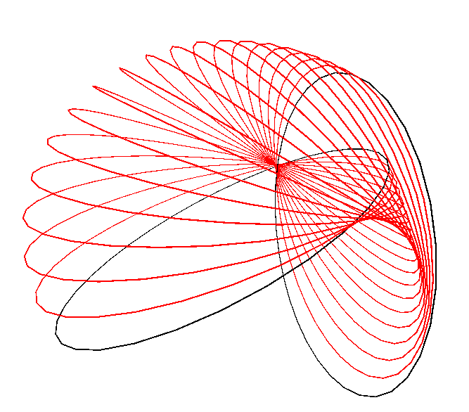
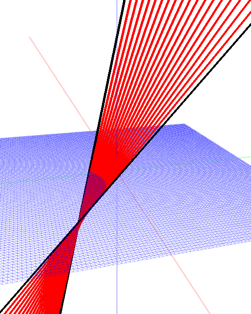
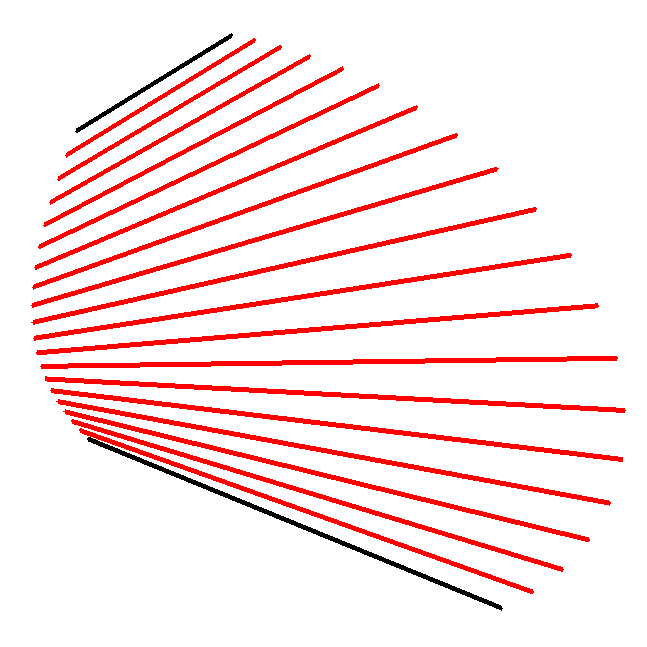
![[*]](footnote.png)


![$[[\Sigma]] = \sqrt{\langle{\Sigma}\rangle_0^2 - \langle{\Sigma}\rangle_4^2}$](img283.svg)
![$\displaystyle \sqrt{\Sigma} = \frac{\Sigma \pm [[\Sigma]]}{\sqrt{2}\sqrt{\langl...
...angle{\Sigma}\rangle_4}{\sqrt{2}\sqrt{\langle{\Sigma}\rangle_0 \pm [[\Sigma]]}}$](img284.svg)


![$\displaystyle R[\alpha X_1 + (1-\alpha)X_2]\tilde{R} = \alpha RX_1\tilde{R} + (1-\alpha)RX_2\tilde{R} $](img293.svg)

![\begin{subfigure}[b]{0.4\textwidth}
\includegraphics[width=\textwidth]{circles.png}
\end{subfigure}](img295.svg)
![\begin{subfigure}[b]{0.4\textwidth}
\includegraphics[width=\textwidth]{pairPair.png}
\end{subfigure}](img296.svg)
![\begin{subfigure}[b]{0.4\textwidth}
\includegraphics[width=\textwidth]{planes.png}
\end{subfigure}](img297.svg)
![\begin{subfigure}[b]{0.4\textwidth}
\includegraphics[width=\textwidth]{spheres.png}
\end{subfigure}](img298.svg)


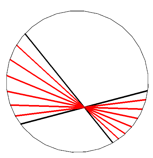
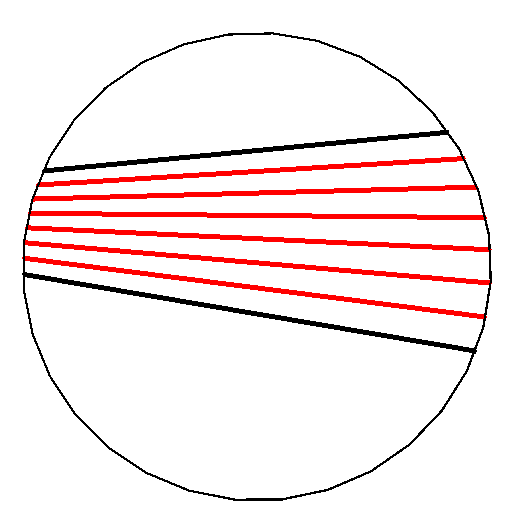

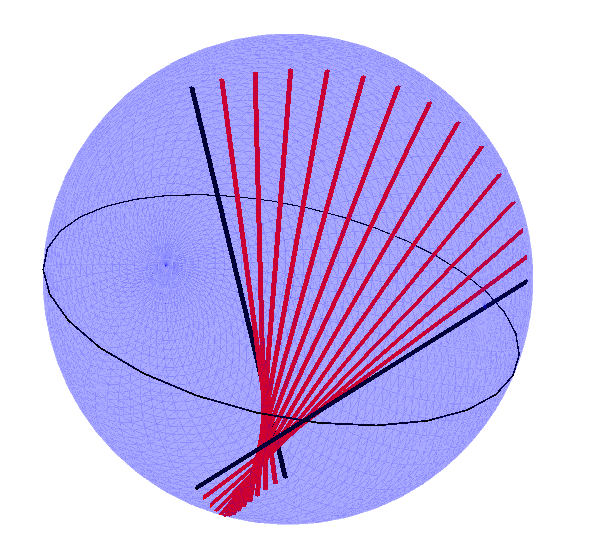


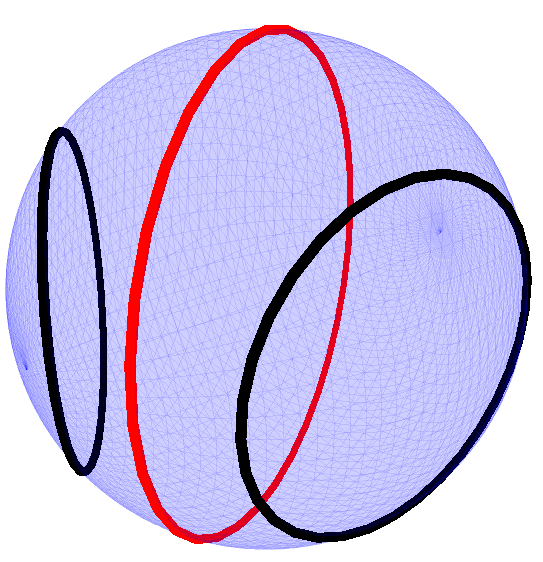
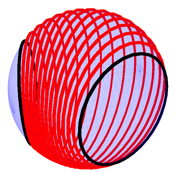


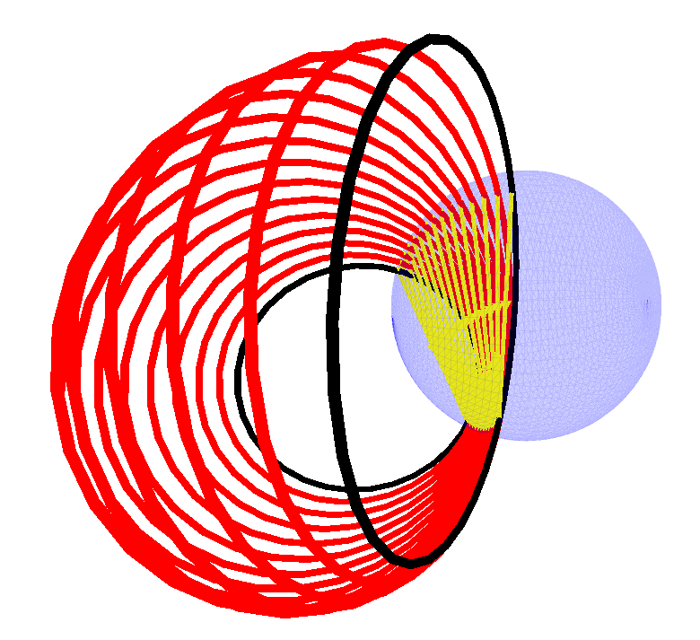


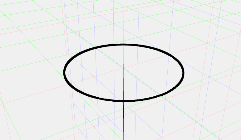


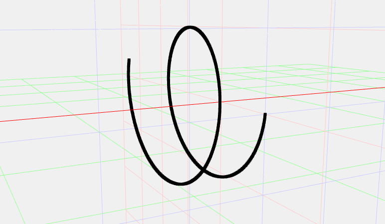


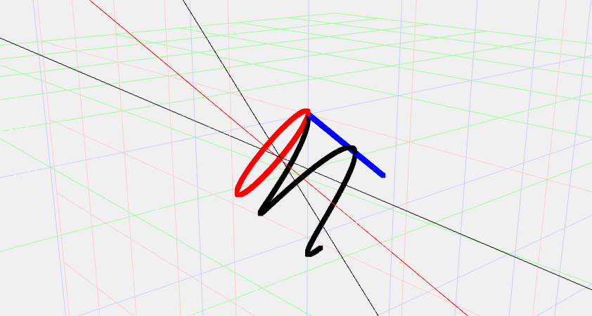


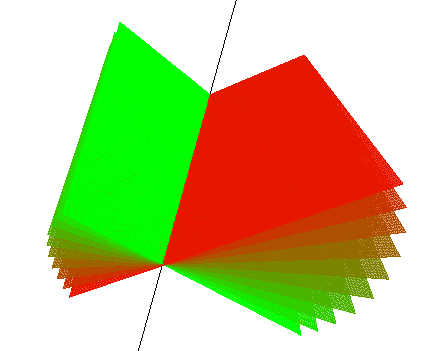
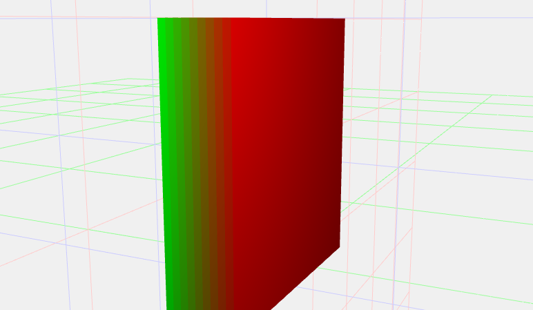
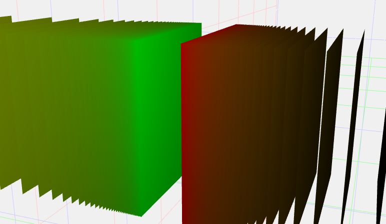


![\begin{subfigure}[b]{0.3\textwidth}
\includegraphics[width=\textwidth]{circle_spline_1.png}
\end{subfigure}](img473.svg)
![\begin{subfigure}[b]{0.3\textwidth}
\includegraphics[width=\textwidth]{circle_spline_2.png}
\end{subfigure}](img474.svg)
![\begin{subfigure}[b]{0.3\textwidth}
\includegraphics[width=\textwidth]{circle_spline_3.png}
\end{subfigure}](img475.svg)
![\begin{subfigure}[b]{0.3\textwidth}
\includegraphics[width=\textwidth]{point_pair_spline_1.png}
\end{subfigure}](img476.svg)
![\begin{subfigure}[b]{0.3\textwidth}
\includegraphics[width=\textwidth]{point_pair_spline_2.png}
\end{subfigure}](img477.svg)
![\begin{subfigure}[b]{0.3\textwidth}
\includegraphics[width=\textwidth]{point_pair_spline_3.png}
\end{subfigure}](img478.svg)
![\begin{subfigure}[b]{1.0\textwidth}{
\includegraphics[width=\textwidth]{before_filter.png}
}
\end{subfigure}](img479.svg)
![\begin{subfigure}[b]{1.0\textwidth}{
\includegraphics[width=\textwidth]{after_filter.png}
}
\end{subfigure}](img480.svg)


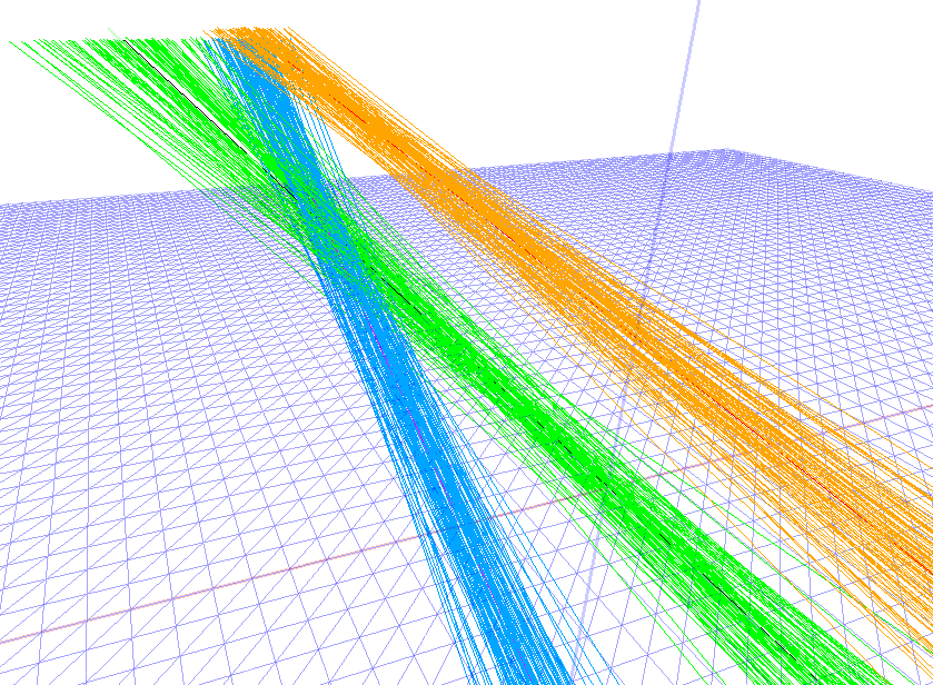
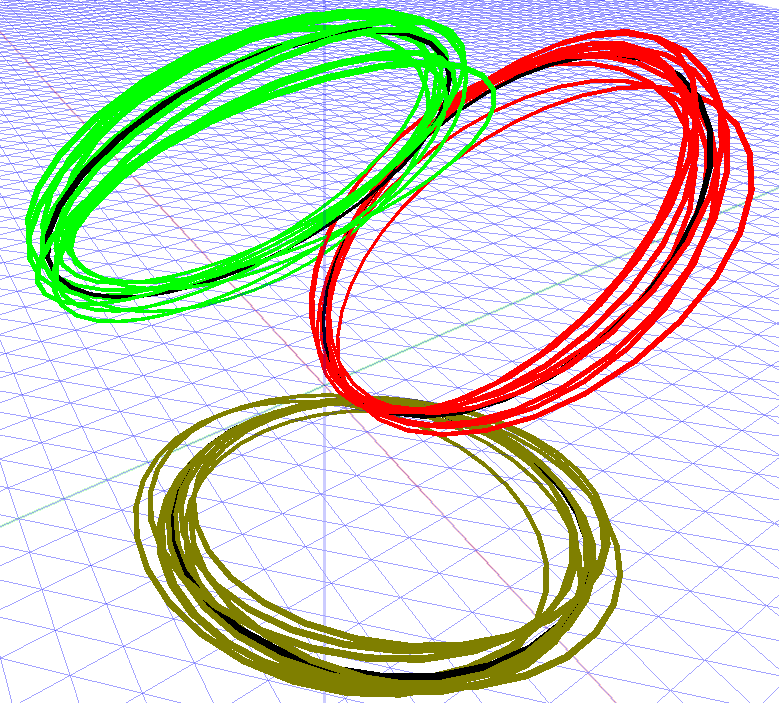


![\includegraphics[width=\textwidth]{FirstFig.eps}](img495.svg)


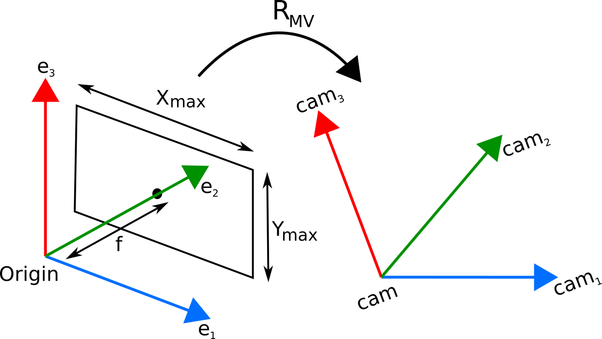 width=
![\includegraphics[width=1.0\textwidth]{226Achawalallobjectsimage.eps}](img508.svg) width=
width=


![\includegraphics[width=0.5\textwidth]{226AchawalSphereIntersection.eps}](img541.svg)


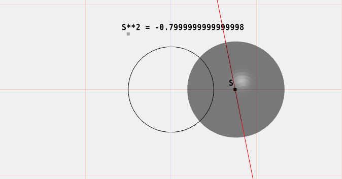
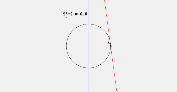
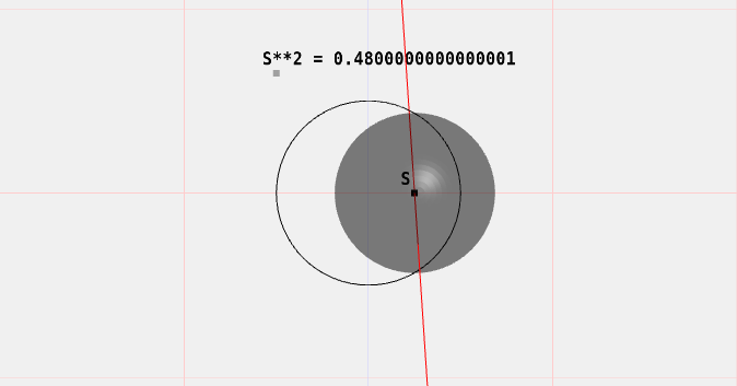 width=


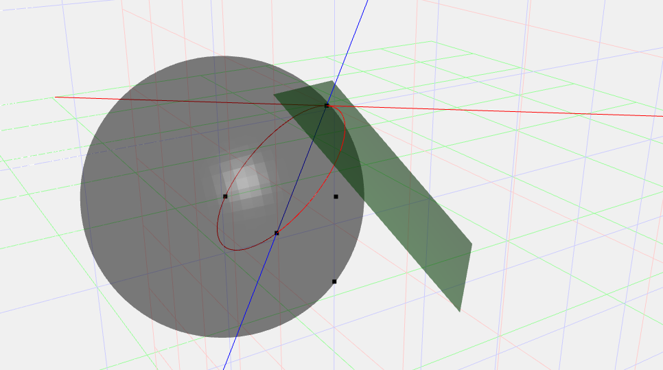


![\includegraphics[scale=0.6]{raytrace.PNG}](img563.svg)
![\includegraphics[scale=0.5]{226AchawalSurfaces.eps}](img564.svg)


![$\displaystyle \sqrt{\Sigma} = \frac{\Sigma + [[\Sigma]]}{\sqrt{2}\sqrt{\langle{...
...langle{\Sigma}\rangle_4}{\sqrt{2}\sqrt{\langle{\Sigma}\rangle_0 + [[\Sigma]]}}.$](img569.svg)


![$\displaystyle C_{\alpha} = \frac{k\mathcal{S}}{(k\mathcal{S})(k\mathcal{S}^{-})}C_\alpha^{'} \equiv \mathcal{S}C_\alpha^{'}, \quad \alpha \in [0,1].$](img577.svg)


![\includegraphics[width=0.8\textwidth]{226AchawalskewIntFinal.eps}](img580.svg)


![$\displaystyle (L\vee[\mathcal{S}C'_\alpha])^2 = 0.
$](img596.svg)


![$\displaystyle \left( L\vee[\langle \sqrt{\Sigma}\rangle _0C'_\alpha] - L\vee[\langle \sqrt{\Sigma}\rangle _4C'_\alpha] \right)^2 = 0.
$](img600.svg)

![$\displaystyle \sqrt{\Sigma} = \frac{\Sigma + [[\Sigma]]}{\sqrt{2}\sqrt{\langle{\Sigma}\rangle_0 + [[\Sigma]]}}
$](img602.svg)
![$\displaystyle \left( L\vee\left[\left\langle \frac{\Sigma + [[\Sigma]]}{\sqrt{2...
...\Sigma}\rangle_0 + [[\Sigma]]}}\right\rangle _4C'_\alpha\right] \right)^2 = 0.
$](img603.svg)
![$\displaystyle \left( L\vee\left[\langle \Sigma + [[\Sigma]]\rangle _0C'_\alpha ...
...vee\left[\langle \Sigma + [[\Sigma]] \rangle _4C'_\alpha\right] \right)^2 = 0.
$](img604.svg)
![$[[\Sigma]]$](img605.svg)
![$\displaystyle \left( L\vee [\langle \Sigma \rangle _0 C'_\alpha]+ [[\Sigma]]L\v...
..._\alpha -
L\vee\left[\langle \Sigma \rangle _4C'_\alpha\right] \right)^2 = 0.
$](img606.svg)
![$\displaystyle =[L\vee (\langle \Sigma\rangle _0C'_\alpha) - L\vee (\langle \Sigma\rangle _4C'_\alpha) ]^2 + [[\Sigma]]^2(L\vee C'_\alpha)^2$](img607.svg)
![$\displaystyle \phantom{=}+[[\Sigma]]\left\{ (L\vee (\langle \Sigma\rangle _0C'_\alpha) - L\vee (\langle \Sigma\rangle _4C'_\alpha))(L\vee C'_\alpha)\right.$](img608.svg)


![$\displaystyle [[\Sigma]] = \sqrt{\langle \Sigma\rangle _0^2 - \langle \Sigma\rangle _4^2} .
$](img614.svg)
![$\displaystyle [L\vee (\langle \Sigma\rangle _0C'_\alpha) - L\vee (\langle \Sigma\rangle _4C'_\alpha) ]^2 + [[\Sigma]]^2(L\vee C'_\alpha)^2$](img615.svg)
![$\displaystyle \hspace*{10ex}= -[[\Sigma]] \left\{L\vee (\langle \Sigma\rangle _0C'_\alpha) - L\vee (\langle \Sigma\rangle _4C'_\alpha)\right\}(L\vee C'_\alpha)$](img616.svg)

![$\displaystyle \left([L\vee (\langle \Sigma\rangle _0C'_\alpha) - L\vee (\langle \Sigma\rangle _4C'_\alpha) ]^2 + [[\Sigma]]^2(L\vee C'_\alpha)^2 \right)^2$](img618.svg)
![$\displaystyle \hspace*{10ex} = [[\Sigma]]^2 \left[ \left\{L\vee (\langle \Sigma...
...a) - L\vee (\langle \Sigma\rangle _4C'_\alpha)\right\}(L\vee C'_\alpha)
\right.$](img619.svg)
![$\displaystyle \phantom{=}\hspace*{10ex} \left. + (L\vee C'_\alpha)\left\{L\vee ...
...gle _0C'_\alpha) - L\vee (\langle \Sigma\rangle _4C'_\alpha)\right\} \right]^2.$](img620.svg)


![$(L\vee[\mathcal{S}C'_\alpha])^2$](img624.svg)
![$\vert(L\vee[\mathcal{S}C'_\alpha])^2\vert < \epsilon$](img625.svg)


![$(L\vee[\mathcal{S}C'_\alpha])^2 = 0$](img630.svg)


![$\displaystyle \hspace*{10ex}=\frac{1}{4}\left[ \left( \dot{X}Xn_{\infty}+ n_{\infty}\dot{X}C\right) \left( XCn_{\infty}+ n_{\infty}XC\right) \right]$](img677.svg)
![$\displaystyle \hspace*{10ex}=\frac{1}{4}\left[ \dot{X}Xn_{\infty}XCn_{\infty}+ n_{\infty}\dot{X}Xn_{\infty}XC\right].$](img678.svg)


![$\displaystyle \frac{\partial [[\Sigma]]}{\partial \alpha} =
\frac{
\langle{\fra...
...4\langle{\frac{\partial \Sigma}{\partial \alpha} }\rangle_4
}
{
2 [[\Sigma]]
},$](img693.svg)

![$\displaystyle \frac{\partial }{\partial \alpha} \left( \frac{1}{\sqrt{2}\sqrt{\langle{\Sigma}\rangle_0 + [[\Sigma]]}} \right)$](img695.svg)
![$\displaystyle = \frac{-1}{2\sqrt{2}}(\langle{\Sigma}\rangle_0 + [[\Sigma]])^{-\...
...rtial \alpha} }\rangle_0 + \frac{\partial [[\Sigma]]}{\partial \alpha} \right),$](img696.svg)

![$\displaystyle = \left( \frac{\partial \Sigma}{\partial \alpha} + \frac{\partial...
...t)\left( \frac{1}{\sqrt{2}\sqrt{\langle{\Sigma}\rangle_0 + [[\Sigma]]}} \right)$](img698.svg)
![$\displaystyle \phantom{=}+\left( \Sigma + [[\Sigma]] \right)\frac{\partial }{\p...
...ac{1}{\sqrt{2}\sqrt{\left\langle{\Sigma}\right\rangle_0 + [[\Sigma]]}} \right).$](img699.svg)


![$\displaystyle \frac{\partial \left(\left[\left(\langle \sqrt{\Sigma}\rangle _0 ...
...t{\Sigma}\rangle _4 \right)\sqrt{\Sigma}\right]^{-1}\right)}{\partial \alpha} =$](img705.svg)
![$\displaystyle \hspace*{5ex}\left[\left(\left\langle \frac{\partial \sqrt{\Sigma...
...a}\rangle _4 \right)\frac{\partial \sqrt{\Sigma}}{\partial \alpha} \right] \ast$](img706.svg)
![$\displaystyle \hspace*{45ex}\left[-\left(\langle \sqrt{\Sigma}\rangle _0 - \langle \sqrt{\Sigma}\rangle _4 \right)\sqrt{\Sigma}\right]^{-2}$](img707.svg)

![$\displaystyle =\left(\left\langle \frac{\partial \sqrt{\Sigma}}{\partial \alpha...
...a}\rangle _0 - \langle \sqrt{\Sigma}\rangle _4 \right)\sqrt{\Sigma}\right]^{-1}$](img709.svg)
![$\displaystyle \phantom{=}\hspace*{5ex}+\left(\langle \sqrt{\Sigma}\rangle _0 - ...
...t{\Sigma}\rangle _4 \right)\sqrt{\Sigma}\right]^{-1}\right)}{\partial \alpha} .$](img710.svg)


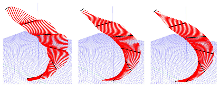


![$\displaystyle L\vee [\mathcal{S}P'_\alpha] = 0.
$](img717.svg)

![$\displaystyle L\vee\left[\frac{ \langle \sqrt{\Sigma}\rangle _0 - \langle \sqrt...
...- \langle \sqrt{\Sigma}\rangle _4 \right)\sqrt{\Sigma}} P'_\alpha\right] = 0.
$](img719.svg)
![$\displaystyle L\vee[\langle \sqrt{\Sigma}\rangle _0P'_\alpha] - L\vee[\langle \sqrt{\Sigma}\rangle _4P'_\alpha] = 0,$](img720.svg)
![$\displaystyle L\vee\left[\left\langle \frac{\Sigma + [[\Sigma]]}{\sqrt{2}\sqrt{...
...rt{\langle{\Sigma}\rangle_0 + [[\Sigma]]}}\right\rangle _4P'_\alpha\right] = 0,$](img721.svg)
![$\displaystyle \left( L\vee [\langle \Sigma \rangle _0 P'_\alpha]+ [[\Sigma]]L\vee P'_\alpha - L\vee\left[\langle \Sigma \rangle _4P'_\alpha\right] \right)^2 = 0.$](img722.svg)
![$\displaystyle L\vee [\langle \Sigma \rangle _0 P'_\alpha] -
L\vee\left[\langle \Sigma \rangle _4P'_\alpha\right] = -[[\Sigma]]L\vee P'_\alpha.
$](img723.svg)
![$\displaystyle (L\vee [\langle \Sigma \rangle _0 P'_\alpha] -
L\vee\left[\langle \Sigma \rangle _4P'_\alpha\right])^2 = [[\Sigma]]^2(L\vee P'_\alpha)^2.
$](img724.svg)

![$\displaystyle (L\vee [\langle \Sigma \rangle _0 P'_\alpha] -
L\vee\left[\langle \Sigma \rangle _4P'_\alpha\right])^2 - [[\Sigma]]^2(L\vee P'_\alpha)^2 = 0,$](img726.svg)


![$\displaystyle S^*\cdot X = [(P_1\wedge P_2)I_5]\cdot X > 0.
$](img730.svg)

![\includegraphics[width=0.4\textwidth]{pntpairsurf.PNG}](img732.svg)
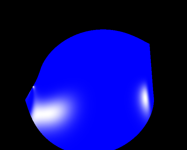


![\includegraphics[width=0.45\textwidth]{triangular_scene.PNG}](img739.svg)
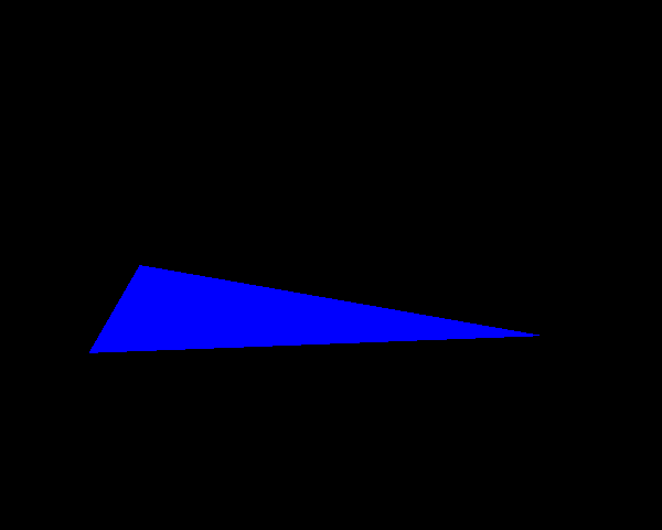


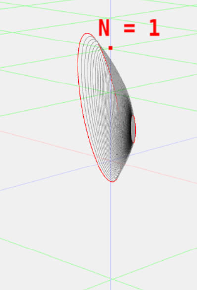 [Order 2]
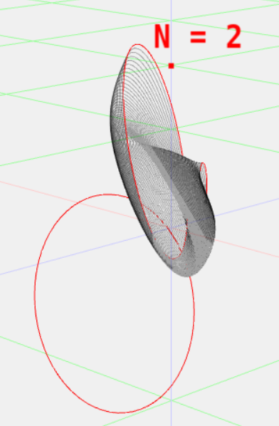 [Order 3]
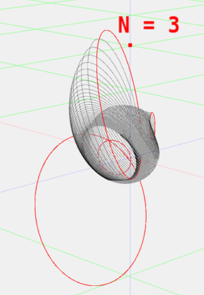


 where
where


![\begin{multline}
\frac{\partial C'_\alpha}{\partial \alpha} = \frac{1}{
[\sum_{i...
...^N \frac{\partial b_{i,N}}{\partial \alpha} w_i
\right]
\right).
\end{multline}](img754.svg)
![$\alpha \in [0,1]$](img755.svg)


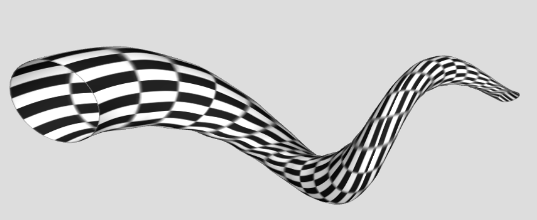

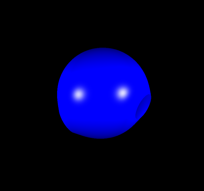
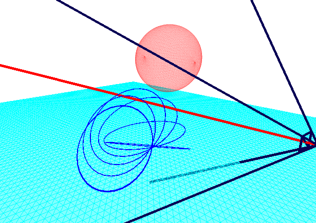
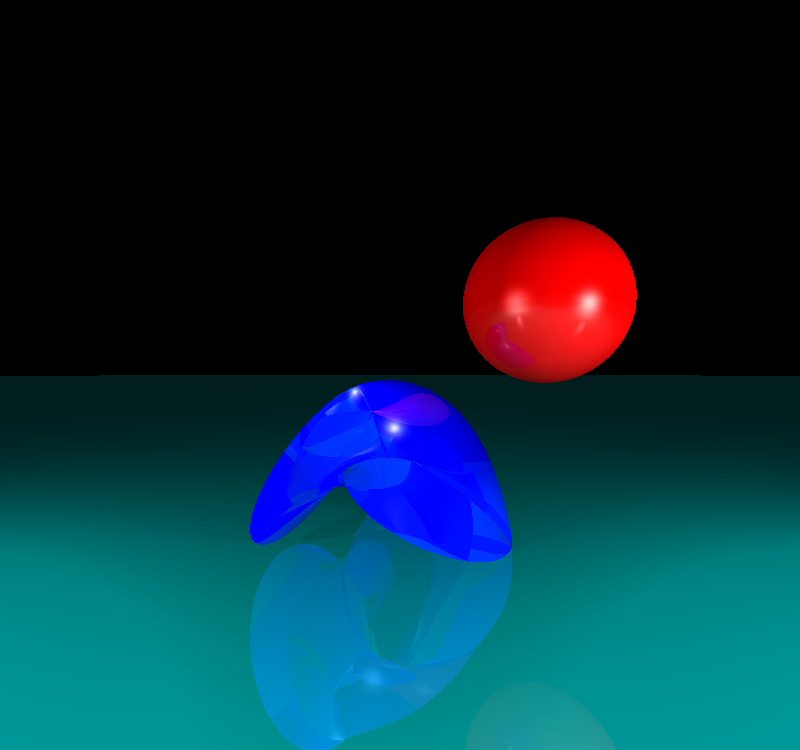


![\includegraphics[width=1.0\textwidth]{mesh_circles.PNG}](img802.svg)
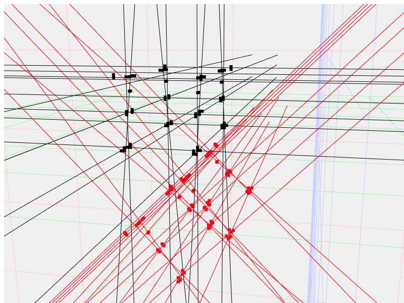
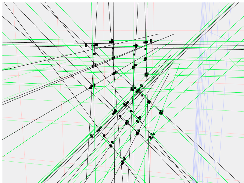


![$\displaystyle M_i = \argmin_j{[C(R_{ij})]}
$](img808.svg)

![\begin{algorithm}
% latex2html id marker 5557
[H]
\SetAlgoLined
\KwResult{$R_e$}...
...k on itself\;
}
}
\caption{Direct rotor estimation algorithm}
\end{algorithm}](img810.svg)
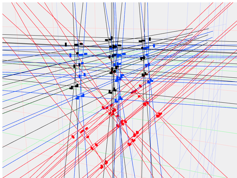
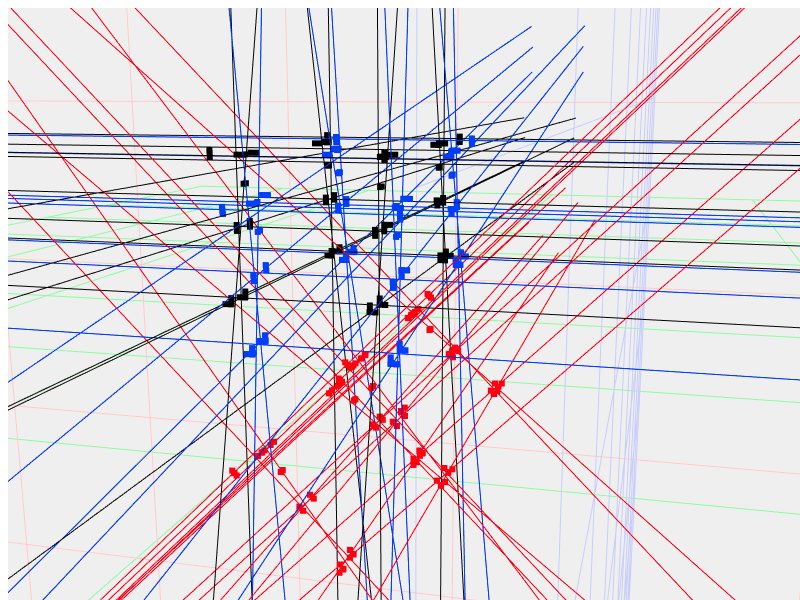
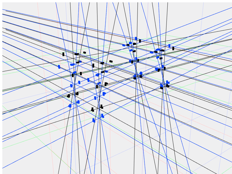
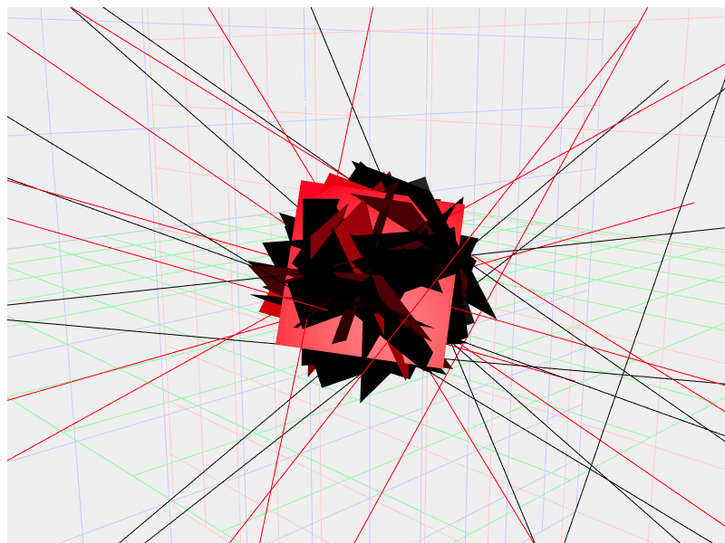


 up
up up
up


![$\displaystyle -ac - (bc + ad)I_3n_{\infty}= [-a\cdot c -a\wedge c] - [(b\cdot c + a \cdot d + b\wedge c + a\wedge d)I_3n_{\infty}].
$](img853.svg)
![$\displaystyle ST = [-a\cdot c]+ [-a\wedge c -(b\wedge c + a\wedge d)I_3n_{\infty}]
+ [-(b\cdot c + a \cdot d )I_3n_{\infty}],
$](img854.svg)


![$\displaystyle \Psi = Q[\Omega_w] .
$](img927.svg)
![$\displaystyle \dot{X} = X \times \Omega_w = X \times Q^{-1}[\Psi] .
$](img928.svg)

![$\displaystyle S_k = [e_1I_3,\,\, e_2I_3,\,\, e_3I_3,\,\, e_1\wedge n_{\infty},\,\, e_2\wedge n_{\infty},\,\, e_3\wedge n_{\infty}] ,
$](img938.svg)
![$\displaystyle S^i = [-e_1I_3,\,\, -e_2I_3,\,\, -e_3I_3,\,\, e_1\wedge n_0,\,\, e_2\wedge n_0,\,\, e_3\wedge n_0]
$](img939.svg)


![$\displaystyle \left(\frac{f}{m} \cdot x\right)n_{\infty}+ \frac{f}{m} = \left(\...
...+ x + n_0\right) \times \sum_i \left[ (S^i\cdot W) \sum_k c_{ik} S_k \right].
$](img952.svg)
![$\displaystyle \sum_i \left[ (S^i\cdot W) \sum_k c_{ik} S_k \right]
$](img953.svg)
![$\displaystyle \sum_i \left[ (S^i\cdot W) \sum_k c_{ik} S_k \right] = \sum_j f_j \left[\sum_k c_{jk} S_k \right] = \sum_j \sum_k f_j c_{jk} S_k
$](img958.svg)


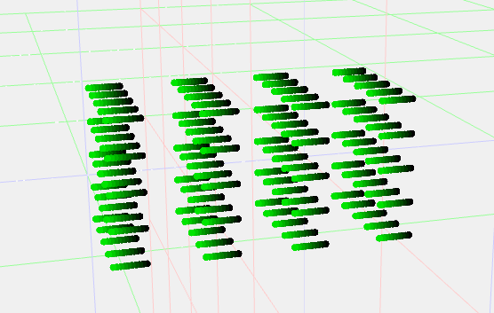
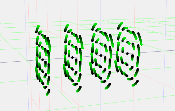


![$\displaystyle (\left(-I_3((\mathcal{M}_a^{-1}t) \wedge x)\right) \cdot x) n_{\i...
..._{\infty}+ x + n_0\right) \cdot \sum_{i \in [4,5,6]} \sum_k t_{i-3} c_{ik} S_k
$](img995.svg)
![$\displaystyle -I_3((\mathcal{M}_a^{-1}t) \wedge x) = \sum_{i \in [4,5,6]} \sum_k t_{i-3} c_{ik} \left(\frac{1}{2}x^2n_{\infty}+ x + n_0\right) \cdot S_k.
$](img997.svg)
![$\displaystyle -I_3((\mathcal{M}_a^{-1}t) \wedge x) = \sum_{i \in [4,5,6]}$](img998.svg)


![$\displaystyle -I_3((\mathcal{M}_a^{-1}t) \wedge x) = \sum_{i \in [4,5,6]} t_{i-3} (c_{i1} x \cdot (e_1I_3) + c_{i2}x \cdot (e_2I_3) + c_{i3} x \cdot (e_3I_3)) .
$](img1002.svg)
![$\displaystyle \sum_{i \in [4,5,6]} -I_3((\mathcal{M}_a^{-1}t_{i-3}e_{i-3}) \wed...
...} (c_{i1} x \cdot (e_1I_3) + c_{i2}x \cdot (e_2I_3) + c_{i3} x \cdot (e_3I_3))
$](img1003.svg)


![$\displaystyle \Psi = Q(\Omega) = m\sum_{i=1}^{i=3} \left[ (\Omega\cdot t^i)l_i + \gamma_i(\Omega\cdot l^i)t_i \right]
$](img1030.svg)
![$\displaystyle Q^{-1}(\Psi) = \Omega = \frac{1}{m}\sum_{i=1}^{i=3}\left[ \frac{1}{\gamma_i}(\Psi\cdot t^i)l_i + (\Psi\cdot l^i)t_i \right] .
$](img1031.svg)


![$\displaystyle \Psi = Q(\Omega) = -m\sum_{i=1}^{i=3} \left[ \langle \Omega\wedge...
...angle _{e1230}l^i + \gamma_i\langle \Omega\wedge t^i\rangle _{e1230}t^i\right]
$](img1067.svg)
![$\displaystyle Q^{-1}(\Psi) = \Omega = -\frac{1}{m}\sum_{i=1}^{i=3}\left[
\fra...
...e l^i\rangle _{e1230}l^i + \langle \Psi\wedge t^i\rangle _{e1230}t^i
\right] .
$](img1068.svg)
![$\displaystyle \Psi = Q(\Omega) = A[J(\Omega)] .
$](img1069.svg)

![$\displaystyle Q_B^{-1}(\Psi_B) = \Omega_B = \frac{1}{m}\sum_{i=1}^{i=3}\left[ \frac{1}{\gamma_i}(\Psi_B \cdot t^i)l_i + (\Psi_B \cdot l^i)t_i \right] .
$](img1077.svg)
![$\displaystyle Q_W^{-1}(\Psi) = \frac{1}{m}\sum_{i=1}^{i=3}\left[ \frac{1}{\gamm...
...ilde{R}) + ((R\Psi_B\tilde{R}) \cdot (Rl^i\tilde{R}))(Rt_i\tilde{R}) \right] .
$](img1081.svg)
![$\displaystyle Q_W^{-1}(\Psi) = \frac{1}{m}\sum_{i=1}^{i=3}\left[ \frac{1}{\gamm...
...(\Psi_B\cdot t^i)(Rl_i\tilde{R}) + (\Psi_B \cdot l^i)(Rt_i\tilde{R}) \right] .
$](img1084.svg)

![$\displaystyle = R\left(\frac{1}{m}\sum_{i=1}^{i=3}\left[ \frac{1}{\gamma_i}(\Psi_B\cdot t^i)l_i + (\Psi_B \cdot l^i)t_i) \right]\right)\tilde{R}$](img1086.svg)

![$\displaystyle Q_W^{-1}(\Psi) = -\frac{1}{m}\sum_{i=1}^{i=3}\left[
\frac{1}{\g...
... + \langle \Psi\wedge (Rt^i\tilde{R})\rangle _{e1230}(Rt^i\tilde{R})
\right] .
$](img1089.svg)
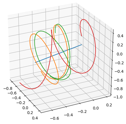


![$\displaystyle \Omega = Q^{-1}[\tilde{R}\Psi R] .
$](img1094.svg)
![$\displaystyle \dot{Y} = \begin{bmatrix}
\dot{R}\\
\dot{\Psi}
\end{bmatrix} = \...
...matrix}
-\frac{1}{2}RQ^{-1}[\tilde{R}\Psi R]\\
RW_{b}\tilde{R}
\end{bmatrix}.
$](img1095.svg)


![$\displaystyle \dot{\Omega} = Q^{-1}[\dot{\tilde{R}}\Psi R + W_b + \tilde{R}\Psi\dot{R}] ,
$](img1101.svg)


![$\displaystyle Q^{-1}[\dot{\tilde{R}}\Psi R + W_b + \tilde{R}\Psi\dot{R}]\wedge(...
... - \Omega\wedge\left(\dot{\tilde{R}}TR + \tilde{R}(\dot{T}R + T\dot{R})\right)
$](img1104.svg)
![$\displaystyle Q^{-1}[W_b]\wedge(\tilde{R}TR) + Q^{-1}[\dot{\tilde{R}}\Psi R + \...
... - \Omega\wedge\left(\dot{\tilde{R}}TR + \tilde{R}(\dot{T}R + T\dot{R})\right)
$](img1105.svg)
![$\displaystyle Q^{-1}[W_b]\wedge(\tilde{R}TR) = - Q^{-1}[\dot{\tilde{R}}\Psi R +...
... - \Omega\wedge\left(\dot{\tilde{R}}TR + \tilde{R}(\dot{T}R + T\dot{R})\right)
$](img1106.svg)
![$\displaystyle Q^{-1}[W_b]\wedge(\tilde{R}TR) = - Q^{-1}[\dot{\tilde{R}}\Psi R +...
...tilde{R}TR) - \Omega\wedge\left(\dot{\tilde{R}}TR + \tilde{R}T\dot{R}\right) .
$](img1108.svg)


![$\displaystyle Q^{-1}[W_b]\wedge(\tilde{R}TR) = - Q^{-1}[\dot{\tilde{R}}\Psi R +...
... - \Omega\wedge\left(\dot{\tilde{R}}TR + \tilde{R}(\dot{T}R + T\dot{R})\right)
$](img1114.svg)


![$\displaystyle \dot{\Omega} = Q^{-1}[\dot{\tilde{R}}\Psi R + \tilde{R}\dot{\Psi}R + \tilde{R}\Psi\dot{R}]
$](img1133.svg)
![$\displaystyle LHS =-\frac{1}{2}\left( Q^{-1}[\dot{\tilde{R}}\Psi R + \tilde{R}\...
...( Q^{-1}[\dot{\tilde{R}}\Psi R + \tilde{R}\Psi\dot{R}] + Q^{-1}[W_b] \right) .
$](img1136.svg)
![$\displaystyle = -\frac{1}{2}Q^{-1}[W_b]U + \frac{1}{2}UQ^{-1}[W_b] + \left( -\f...
...]U + \frac{1}{2}U Q^{-1}[\dot{\tilde{R}}\Psi R + \tilde{R}\Psi\dot{R}] \right)
$](img1137.svg)


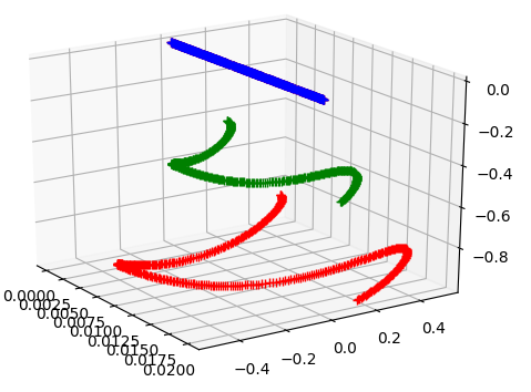
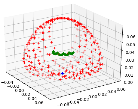
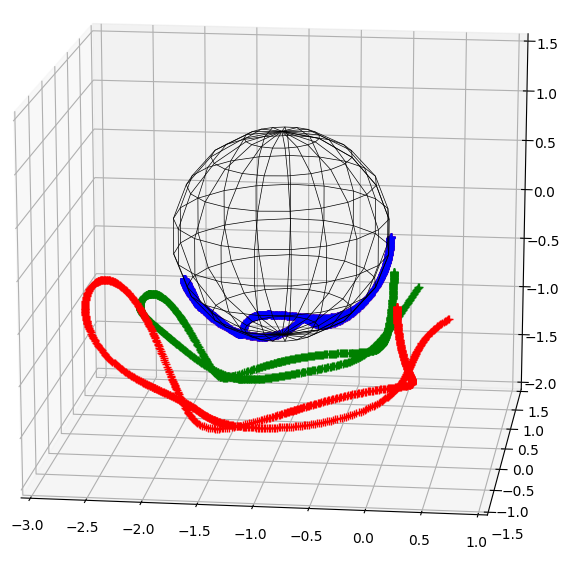
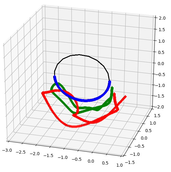


![$\displaystyle = Q^{-1}[W_b]\times (\tilde{R}VR) + Q^{-1}[\dot{\tilde{R}}\Psi R ...
...frac{1}{2}\tilde{\Omega}\dot{\tilde{R}}VR - \frac{1}{2}\tilde{R}V\dot{R}\Omega
$](img1159.svg)
![$\displaystyle = Q^{-1}[F]\times (\tilde{R}VR) + Q^{-1}[S]\times (\tilde{R}VR) +...
...frac{1}{2}\tilde{\Omega}\dot{\tilde{R}}VR - \frac{1}{2}\tilde{R}V\dot{R}\Omega
$](img1160.svg)
![$\displaystyle (\tilde{R}VR) \times Q^{-1}[F]
= - \ddot{U} +
Q^{-1}[S]\times (...
...e{R}}(\dot{V}R + V\dot{R})
+ \tilde{R}\ddot{V}R + 2\tilde{R}\dot{V}\dot{R}
$](img1161.svg)
![$\displaystyle + Q^{-1}[\dot{\tilde{R}}\Psi R + \tilde{R}\Psi\dot{R}] \times (\t...
...ac{1}{2}\tilde{\Omega}\dot{\tilde{R}}VR - \frac{1}{2}\tilde{R}V\dot{R}\Omega.
$](img1162.svg)
![$\displaystyle U = A\left[\tilde{R}VR\right], \,\,\,\,\,\,\,\, \dot{U} = A\left[\dot{\tilde{R}}VR + \tilde{R}(\dot{V}R + V\dot{R})\right] ,$](img1166.svg)
![$\displaystyle \ddot{U} = A\left[ \ddot{\tilde{R}}VR
+ 2\dot{\tilde{R}}(\dot{V}R...
...
+ \tilde{R}\ddot{V}R + 2\tilde{R}\dot{V}\dot{R} + \tilde{R}V\ddot{R} \right] .$](img1167.svg)
![$\displaystyle A\left[ \ddot{\tilde{R}}VR + \tilde{R}V\ddot{R}\right] =
A\left[ ...
...V\dot{R})
- \tilde{R}\ddot{V}R - 2\tilde{R}\dot{V}\dot{R} \right] + \ddot{U}
$](img1168.svg)
![$\displaystyle A\left[(\tilde{R}VR)\times Q^{-1}[F]\right] = A\left[-((\tilde{R}...
...n of }R, \Psi, U, \dot{U}, \ddot{U}, V, \dot{V}, \ddot{V} \right] - \ddot{U} .
$](img1169.svg)


![$\displaystyle \dot{\Phi} = \Omega_w + \frac{1}{2}\Phi\times\Omega_w + \left(\fr...
...heta\vert(\cos{\vert\theta\vert} - 1)} \right)\Phi\times [\Phi \times \Omega_w]$](img1173.svg)
![$\displaystyle + \left(\frac{1}{\vert\theta\vert^4} + \frac{\vert\theta\vert + \...
...t} - 1)} \right) \Phi \times [\Phi \times [\Phi \times [\Phi \times \Omega_w]]]$](img1174.svg)


![\includegraphics[width=0.8\textwidth]{frames.pdf}](img1228.svg)


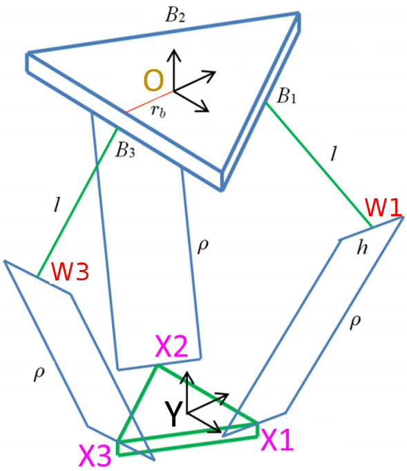
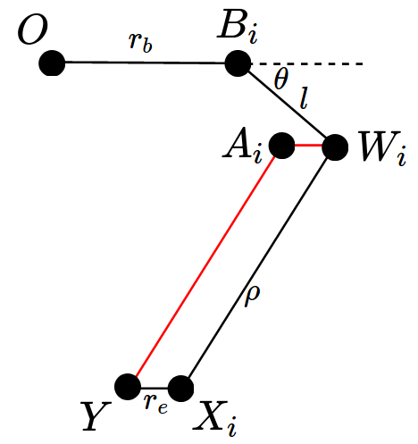
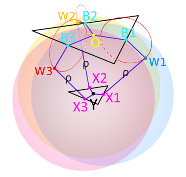


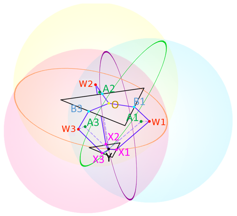


![\includegraphics[width=0.8\textwidth]{DeltaScrews.pdf}](img1351.svg)


![$\displaystyle \begin{bmatrix}
\dot{y}_{e_1} \\
\dot{y}_{e_2} \\
\dot{y}_{e_3}...
...]) & ...
\end{bmatrix}\begin{bmatrix}
... \\
\Omega_{10} \\
...
\end{bmatrix}$](img1391.svg)