Wide Angle Lens Distortion
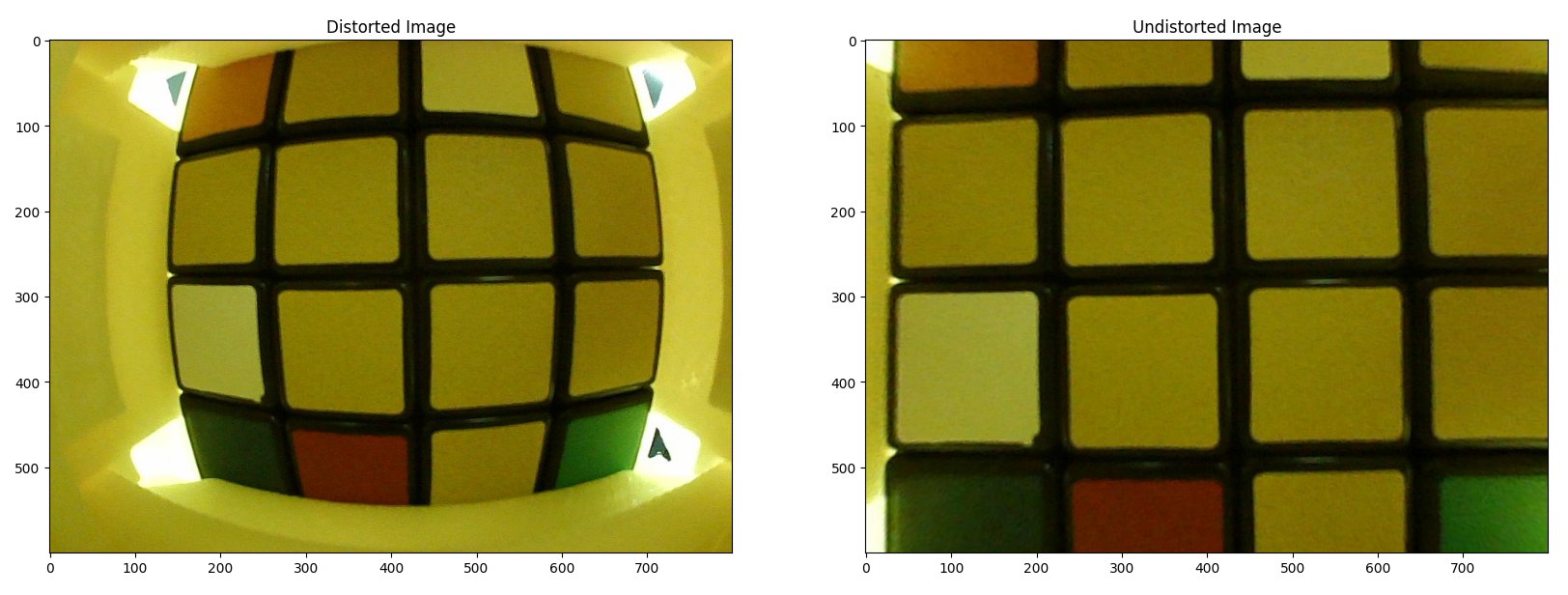
When a human looks at an image that is distorted with a wide angle lens, we can tell pretty much immediately that the image is distorted. Specifically we can tell that objects with straight lines in the 3D world do not have straight lines in the image. In almost all computer vision applications, we want to correct this distortion before we do anything else. But how exactly do we go about making straight-lines straight again?
Simple Radial Undistortion Models
To actually estimate undistortion we will need to have a model to fit to our distorted image. Mathematically one of the simplest ways to describe a lens undistortion model is simply to use some form of spherically symetric function that operates on pixel coordinates. If we define our distorted pixels as $(u', v')$ our undistorted pixels as $(u, v)$ and the centre of image distortion as $(c_x, c_y)$ then we can write a general radially symmetric undistortion model as:
$$\begin{aligned} & r = \sqrt{(u' - c_x)^2 + (v' - c_y)^2} \\ & u = f(r) (u' - c_x) + c_x \\ & v = f(r) (v' - c_y) + c_y \end{aligned}$$Where $f(r)$ is some 1D function of $r$ that we can use to model the required undistortion in the image.
There are many different possible functions that we could use for $f(r)$ but one of the simplest and most effective is a polynomial division model:
$$\begin{aligned} & d(r) = \frac{1}{1 + d_1 r^2 + d_2 r^4} \\ \\ & u = d(r) (u' - c_x) + c_x \\ & v = d(r) (v' - c_y) + c_y \end{aligned}$$This polynomial division model is symmetric about the origin and has two parameters $d_1$ and $d_2$. By adjusting these parameters we can model a wide range of different amounts of distortion.
Estimating Distortion by Straighting Lines
One way to estimate the distortion in an image is to use straight lines. We can use the fact that straight lines in the 3D world should be straight in the image to estimate the distortion.
If we can evaluate how "straight-line-y" our image is then we can use this in a non-linear optmisation process to tweak our undistortion process until we have the most "straight-line-y" image, ie. the best possible undistorted image.
So how can we measure how full of straight lines an image is?
Traditional computer vision and image processing folks will be well aware of the
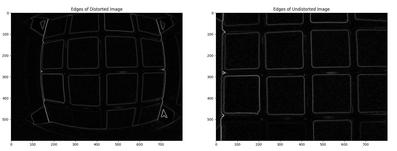
To detect lines in an image with these transforms, the first thing we need to do is to compute the edges of the image. My personal favourite way to do this is by convolution use the Sobel filter. The Sobel filter is a convolution filter that computes the gradient of the image. It's fast, easy to use and gives good results. Below is the original image and the result of applying the Sobel filter to it.
The following code is used to compute the edges and Radon transform of the images and plot the results.
    import cv2
    from skimage.transform import radon
    import matplotlib.pyplot as plt

    # Load the distorted and undistorted image
    distorted_image = cv2.imread('distorted_image.png', cv2.IMREAD_COLOR)
    undistorted_image = cv2.imread('undistorted_image.png', cv2.IMREAD_COLOR)
    distorted_image_gray = np.array(cv2.cvtColor(distorted_image, cv2.COLOR_BGR2GRAY), dtype=np.float64)
    undistorted_image_gray = np.array(cv2.cvtColor(undistorted_image, cv2.COLOR_BGR2GRAY), dtype=np.float64)

    # Convolve with the sobel filter to get the edges
    def compute_edge_intensity(image_gray: np.ndarray) -> np.ndarray:
        """
        Compute the edge intensity of the image using the Sobel filter.
        """
        x = cv2.Sobel(image_gray, cv2.CV_64F, 1, 0, ksize=3)
        y = cv2.Sobel(image_gray, cv2.CV_64F, 0, 1, ksize=3)
        return np.sqrt(x**2 + y**2)

    print("Computing edges of the images")
    distorted_image_edges = compute_edge_intensity(distorted_image_gray)
    undistorted_image_edges = compute_edge_intensity(undistorted_image_gray)

    # Compute the Radon transform of the images
    print("Computing Radon transform of the images")
    theta = np.linspace(0.0, 180.0, max(image.shape), endpoint=False)
    radon_distorted = radon(distorted_image_edges, theta=theta, circle=False)
    radon_undistorted = radon(undistorted_image_edges, theta=theta, circle=False)

    # Normalize the Radon transform
    radon_distorted = radon_distorted/np.max(radon_distorted.flatten())
    radon_undistorted = radon_undistorted/np.max(radon_undistorted.flatten())

    # Plot the images
    plt.figure()
    plt.subplot(1, 2, 1)
    plt.imshow(distorted_image)
    plt.title('Distorted Image')
    plt.subplot(1, 2, 2)
    plt.imshow(undistorted_image)
    plt.title('Undistorted Image')
    plt.tight_layout()

    # Plot the edges of the images
    plt.figure()
    plt.subplot(1, 2, 1)
    plt.imshow(distorted_image_edges, cmap='gray')
    plt.title('Edges of Distorted Image')
    plt.subplot(1, 2, 2)
    plt.imshow(undistorted_image_edges, cmap='gray')
    plt.title('Edges of Undistorted Image')
    plt.tight_layout()

    # Plot the Radon transform of the images
    plt.figure()
    plt.subplot(1, 2, 1)
    plt.imshow(radon_distorted, cmap='gray')
    plt.title('Radon Transform of Distorted Image')
    plt.ylabel('r')
    plt.subplot(1, 2, 2)
    plt.imshow(radon_undistorted, cmap='gray')
    plt.title('Radon Transform of Undistorted Image')
    plt.tight_layout()
    plt.show()
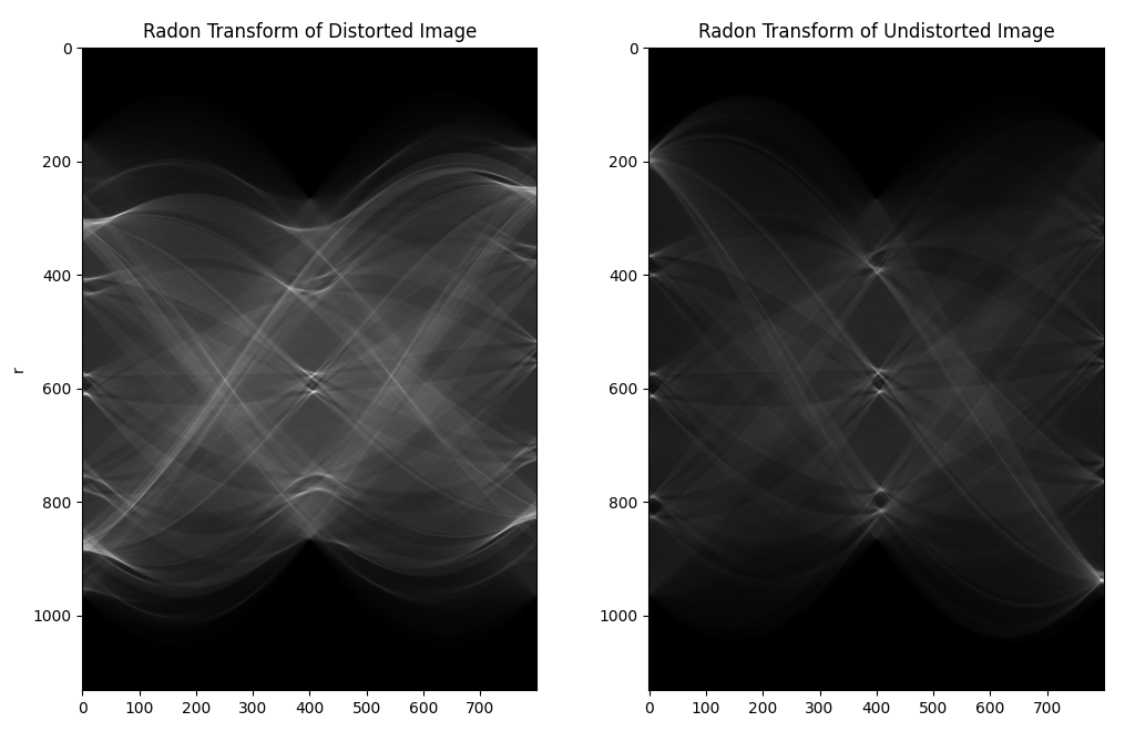
Above is the Radon transform of the distorted and undistorted images, normalised relative to their maximum values. The transform of the distorted image appears on average brighter than the undistorted radon transform which is what we would expect as on average the undistorted radon transform has much sharper peaks.
The Hough transform is similar to the above Radon transform but is used to detect discrete lines in an image rather than transform the image into a different space. It is similar to selecting peaks from the Radon transform and the OpenCV version directly outputs the lines that it detects in the image.
These transforms are all well and good but are there any actual production ready algorithms that use these transforms to estimate straight-line-y-ness? And how do you go from a transform to a number you can actually optimise? For the rest of this blog post we will be considering the model and methods taken from this very interesting paper: An Iterative Optimization Algorithm for Lens Distortion Correction Using Two-Parameter Models.
Breakdown of the Estimation Algorithm
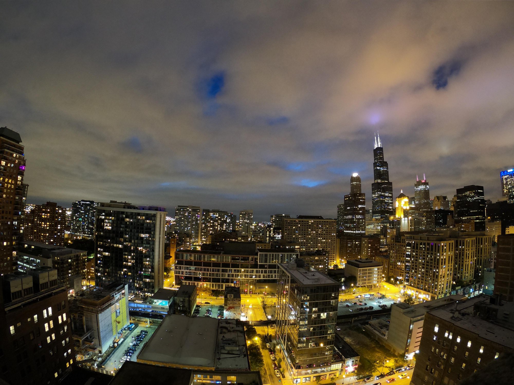
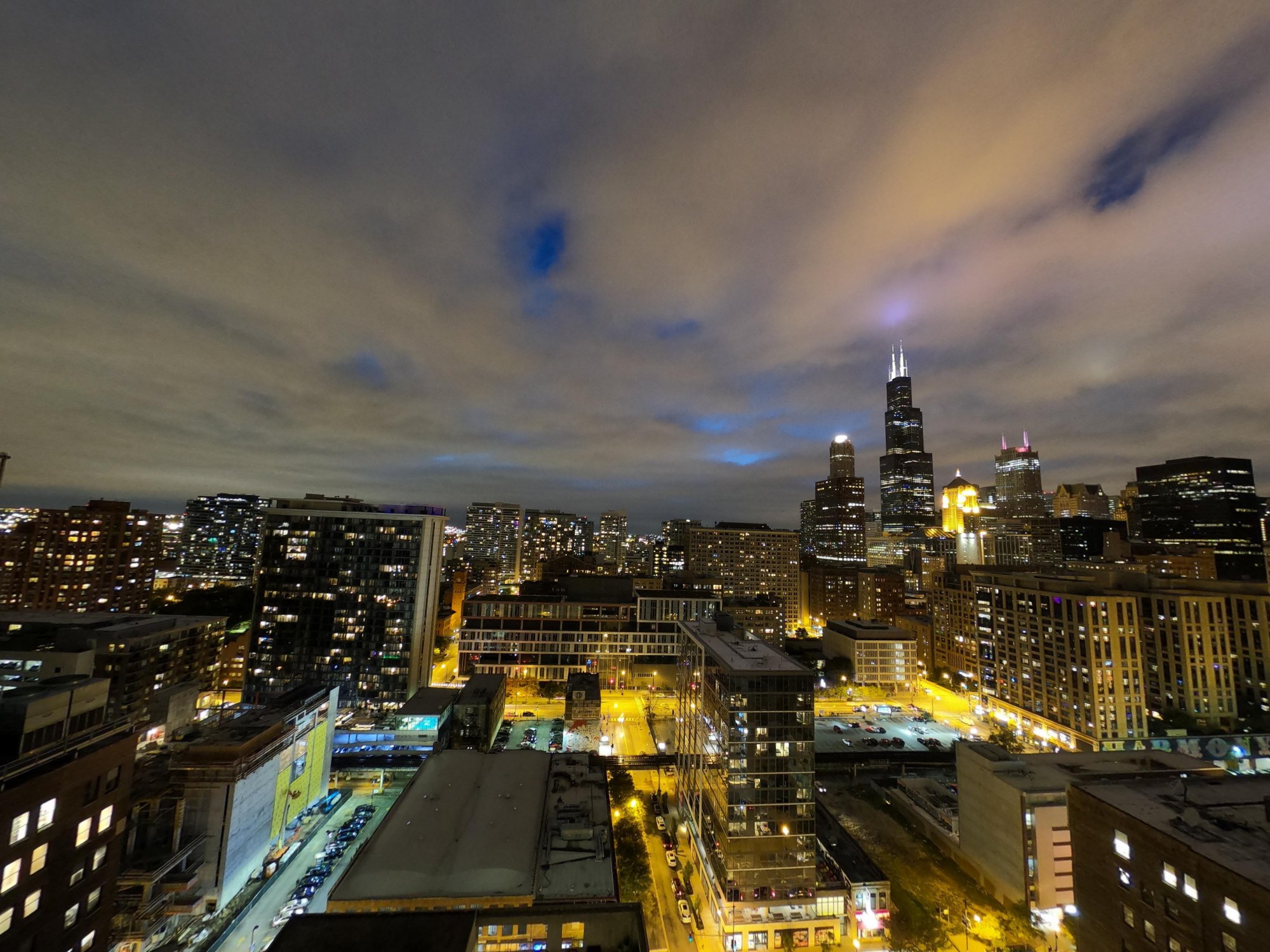
The algorithm from the paper is broken down into several steps. We will work through them showing intermediate results as we go. Let's work with this distorted image of Chicago:
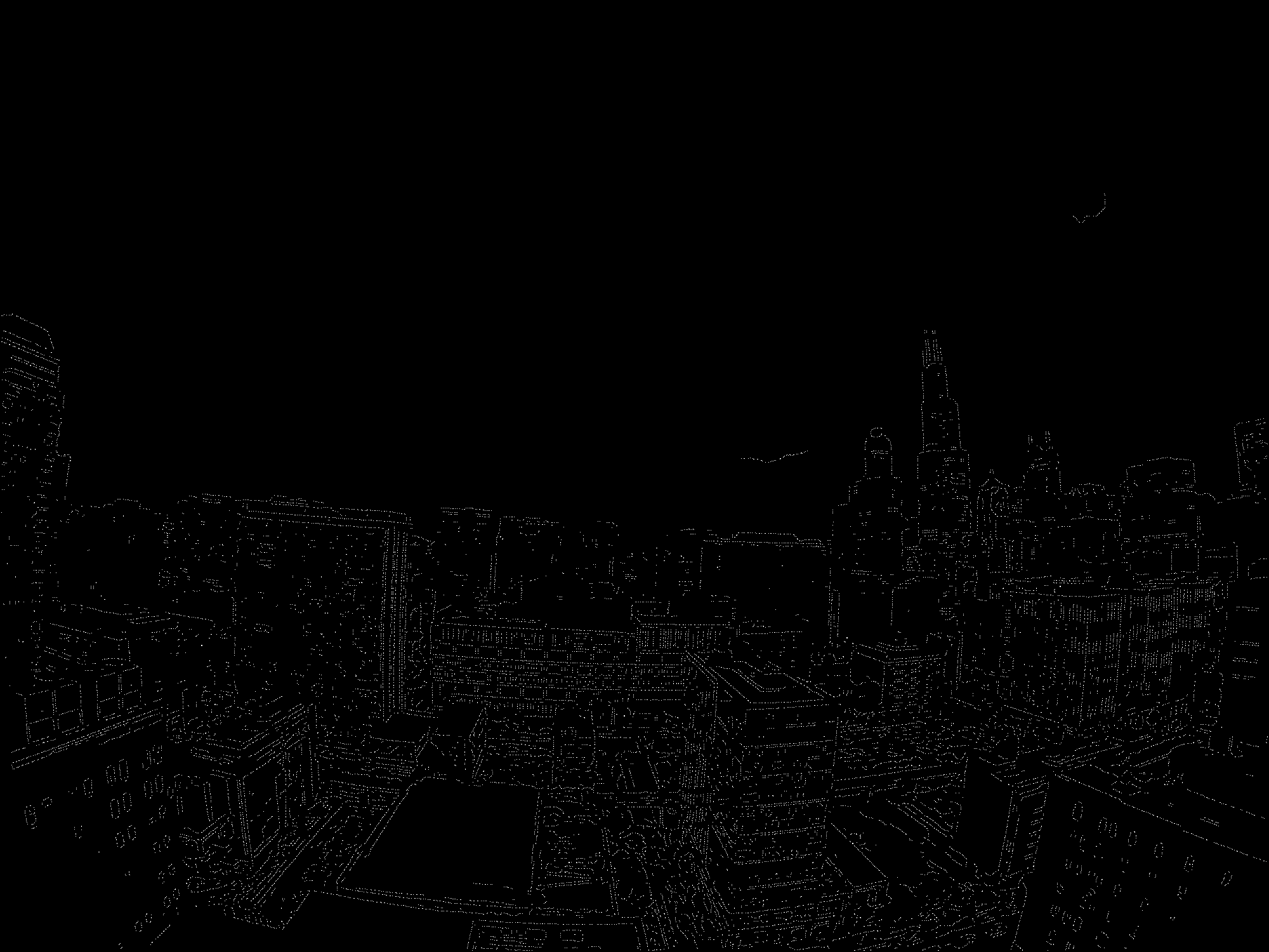
Stage 1: Edge Detection using the Canny Method
The Canny Method is a multi-stage algorithm that detects edges in an image. It is one of the most well known and popular edge detection algorithms. It is implemented in Matlab here and in OpenCV here. However the paper we are looking at today implements it themselves and this allows them a large degree of control over the process. The steps of the Canny method are:
- Gaussian Convolution: Smooth the input image using an approximation of the recursive filter for Gaussian convolution.
- Image Gradient: Compute the image gradient using specific convolution masks to ensure rotation invariance.
- Canny Thresholds: Set the low and high thresholds for the Canny method as percentiles of the gradient norm.
- Non-maximum Suppression: Identify local maxima of the gradient norm in the gradient direction and classify them as edges.
- Hysteresis Implementation: Classify pixels as edges if they are connected to edge pixels, and explore their neighborhoods recursively.
This produces an image that looks like this with individual edge pixels set to 1 and all else set to 0:
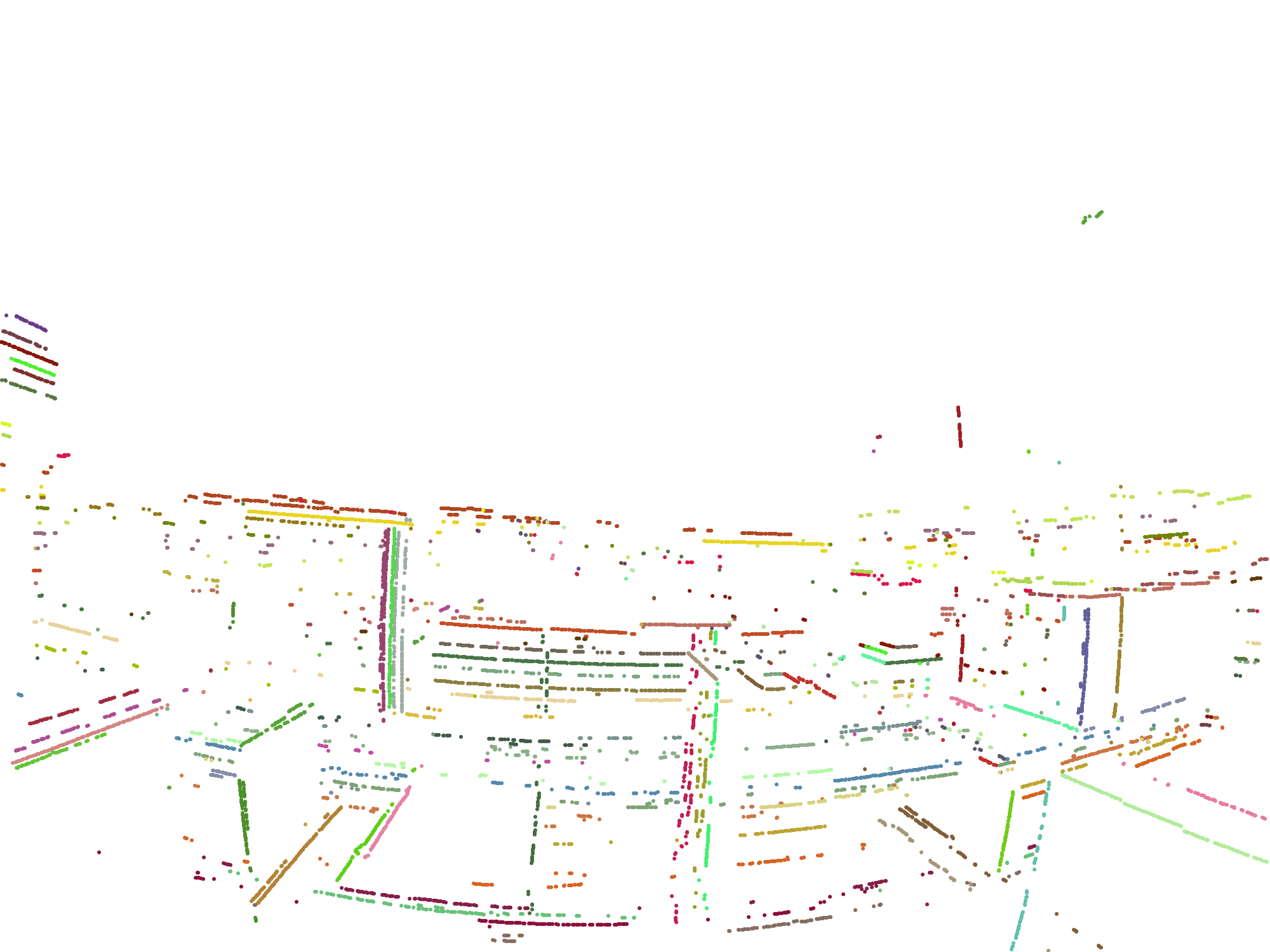
Stage 2: Detect Lines with Improved Hough Transform
With the edges detected the authors of the paper next move onto their Hough transform based line detection algorithm. First of all they defined an extension of the Hough transform to include a curvature parameter. This effectively turns the Hough transform from a line integral transform into a curvature parametrised curve integral transform and by stepping through this parameter the authors of the paper create a 3D output space. Points in this 3D Hough output space map to specific curves in the image (lines in the undistorted space) and using the best lines available from this step the authors are able to estimate a starting point for the first parameter of the undistortion model and the centre of distortion.
- Extract Distortion Model: Extract a one-parameter distortion model and the most voted lines using an extended Hough transform.
- Voting Process: Fill the 3D score volume based on edge points, distance, and angle variations to vote in the Hough space.
- Line Detection: Select lines with the highest votes and refine the points associated with these lines.
This produces an image that looks like this with individual line segements highlighted and ready for undistortion estimation.
Stage 3: Iterative Optimization
With a good starting point for the centre of distortion and the first parameter of the undistortion model the authors start refining the model using a non-linear optimization algorithm. They compute the distance to a straight line for each point associated with a specific line and then optimise the distortion model to minimise this. They then update the point-line associations and repeat the process until there are no changes in the number of points associated with each line.
- Initialize Parameters: Start with initial distortion parameters and center of distortion.
- Gradient and Hessian Calculation: Compute the gradient vector and Hessian matrix for the distortion parameters.
- Iterative Minimization: Use an iterative scheme to minimize the energy function, which reduces the distance from points to lines.
- Model Update: Update the lens distortion model with the optimized parameters.
Stage 4: Image Distortion Correction
Finally with the full distortion model calculated the authors can apply the distortion to the whole original colour image and generate a corrected image.
- Inverse Vector Calculation: Compute the inverse vector for image pixels using the estimated lens distortion model.
- Distortion-Free Image Computation: Apply bilinear interpolation to generate the distortion-free output image based on the corrected pixel coordinates.
We now have an undistorted image, and we didn't have to play around with checkerboards:
Matching Division Model to OpenCV
While it's nice to have an algorithm that can estimate the distortion without needing a specific checkerboard it's generally a good idea to be able to use very popular libraries like OpenCV to do our undistorting for us as these libraries are very widespread in the robotics community and well maintained. If we can convert our division model to the OpenCV model then we can estimate with our Hough code and then store coefficients and undistort with OpenCV.
Lets write out the equations for the two models and then we can compare the similarities and differences between them.
The division model:
$$\begin{aligned} & r = \sqrt{(u' - c_x)^2 + (v' - c_y)^2} \\ & d(r) = \frac{1}{1 + d_1 r^2 + d_2 r^4} \\ \\ & u = d(r) (u' - c_x) + c_x \\ & v = d(r) (v' - c_y) + c_y \end{aligned}$$What do we notice about the division model?
- The division model is a direct correction model; it is a model that is used to correct the distortion that is present in the image by transforming distorted pixels.
- The division model operates in image coordinates. This means that the distortion model is applied after the multiplication by the focal length so the scale of the polynomial is dependent on the focal length.
And now the OpenCV model:
$$\begin{aligned} & r_\theta = \sqrt{x^2 + y^2} \\ & \theta = \arctan(r_\theta) \\ & \theta_d = \theta \left(1 + k_1 \theta^2 + k_2 \theta^4 + k_3 \theta^6 + k_4 \theta^8\right) \\ & s(r_\theta) = \frac{\theta_d}{r_\theta} \\ \\ & u' = s(r_\theta) x f + c_x \\ & v' = s(r_\theta) y f + c_y \end{aligned}$$What do we notice about the OpenCV model?
- The OpenCV model is a distortion model; it is a generative model where the coefficients of the model describe a polynomial that is used to distort rays of light that would otherwise be modeled as projecting onto an image plane as in the pinhole model.
- The OpenCV model operates in normalized image coordinates. This means that the distortion model is applied before multiplication by the focal length so the scale of the polynomial is not dependent on the focal length.
The first thing to do that will make things a lot easier when converting one to the other is to assume that we have centred our image at the principal distortion point, $(c_x, c_y) = (0, 0)$.
We then need to link the two models in terms of a single one of $r$ or $r_\theta$. Let's start with the OpenCV model:
$$\begin{aligned} & r_\theta^2 = x^2 + y^2 \\ & r^2 = u'^2 + v'^2 \\ & u' = s(r_\theta) x f \\ & v' = s(r_\theta) y f \\ & r^2 = \left(s(r_\theta) x f\right)^2 + \left(s(r_\theta) y f\right)^2 \\ & = f^2 s(r_\theta)^2 (x^2 + y^2) \\ & = f^2 s(r_\theta)^2 r_\theta^2 \\ \\ & r = f s(r_\theta) r_\theta \end{aligned}$$We can then also consider the division model:
$$\begin{aligned} & r = \sqrt{u'^2 + v'^2} \\ & d(r) = \frac{1} {(1 + d_1 r^2 + d_2 r^4)} \\ & u = d(r) u' \\ & v = d(r) v' \\ & u^2 + v^2 = d(r)^2 (u'^2 + v'^2) \\ \\ & x f = u \\ & y f = v \\ & u^2 + v^2 = f^2 (x^2 + y^2) \\ \\ & f^2 (x^2 + y^2) = d(r)^2 (u'^2 + v'^2) \\ & f^2 r_\theta^2 = d(r)^2 r^2 \\ & r_\theta^2 = d(r)^2 r^2 / f^2 \\ & r_\theta = d(r) r / f \end{aligned}$$Substituting $r_\theta = d(r) r / f$ into $r = f s(r_\theta) r_\theta$ we get:
$$\begin{aligned} & r = \frac{f s \left( d(r) r / f \right) d(r) r}{ f} \\ & r = s \left( d(r) r / f \right) d(r) r \\ & r \left( s \left( d(r) r / f \right) d(r) - 1 \right) = 0 \\ & s \left( d(r) r / f \right) d(r) - 1 = 0 \\ & s \left( d(r) r / f \right) = \frac{1} {d(r)} \end{aligned}$$This gives us a cost function. We can compute $d(r)$ for a range of $r$ values and then use a non-linear optimization algorithm to find the values of $k_i$ that minimize the cost function.
This is what the code would look like to do this:
def match_opencv_distortion_to_undistortion_model(undistortion_model: Callable, max_r: float):
    """
    Implements fitting s() using the equation:
    s(d(r) * r / f) = 1 / d(r)
    """
    r_array = np.linspace(1.0, max_r, 4000)
    d = np.array([undistortion_model(r) for r in r_array])
    def cost_function(k_array):
        k1, k2, k3, k4 = k_array
        sumout = 0.0
        for i, r in enumerate(r_array):
            r_theta = d[i] * r / DEFAULT_OPENCV_FOCAL_LENGTH
            sumout += (1.0 / d[i] - opencv_fisheye_polynomial(r_theta, k1, k2, k3, k4, opencv_focal_length=1.0))**2
        return sumout
    k0 = [0.0, 0.0, 0.0, 0.0]
    res = minimize(
        cost_function,
        k0,
        method='l-bfgs-b',
        options={'ftol': 1e-10, 'disp': False, 'maxiter': 10000},
    )
    print(res)
    return res.x
We could of course decide to go the other way, given an OpenCV model we could compute $d(r)$ by some more gentle algebra manipulation:
$$\begin{aligned} & r_\theta = d(r) r / f \\ & r = f s(r_\theta) r_\theta \\ & r_\theta = d\left( f s(r_\theta) r_\theta \right) s(r_\theta) r_\theta \end{aligned}$$This gives us a cost function. We can compute $s(r_\theta)$ for a range of $r_\theta$ values and then use a non-linear optimization algorithm to find the values of $d_i$ that minimize the cost function.
Conclusion and Code
In this blog post we have looked at how to estimate lens distortion using straight lines in an image. We have seen how the Radon and Hough transform can be used to detect lines in an image and we have analysed a production system for carrying out lens distortion using straight lines only. If you would like to play around with the code I have added some pybindings to the original C++ code and it is all available on my GitHub.