Automated Derivative Estimation with Kalmangrad
Estimating derivatives from noisy, non-uniformly sampled data is a pervasive challenge in fields like signal processing, control systems, and data analysis. Traditional numerical differentiation methods tend to amplify noise, leading to inaccurate and unreliable results. If you've ever tried to naively differentiate sensor data, you've likely encountered this problem.
Enter Kalmangrad, a Python package that leverages Bayesian filtering techniques to compute smooth, higher-order derivatives of non-uniformly sampled time series data. Built on top of the bayesfilter package, Kalmangrad provides a robust alternative to traditional numerical methods, allowing you to estimate derivatives up to any specified order.
Why Kalmangrad?
Traditional methods for derivative estimation, like finite differences, are highly sensitive to noise and require uniformly sampled data. Kalmangrad overcomes these limitations by:
- Handling Noise Robustly: Uses Bayesian filtering to mitigate the effects of noise in the data.
- Flexible Time Steps: Capable of processing non-uniformly sampled data without the need for resampling.
- Higher-Order Derivatives: Computes derivatives up to any specified order, providing more insights into the dynamics of your data.
- Easy Integration: Offers a simple API for easy integration into existing projects.
- Lightweight: Requires only NumPy and the bayesfilter package, keeping dependencies minimal.
Under the Hood: Bayesian Filtering Approach
Kalmangrad uses a Bayesian filtering framework to estimate derivatives. By modeling the system as a state-space model and applying Kalman filters (and smoothers), it provides a probabilistic estimate of the derivatives, including uncertainties.
The state vector is defined as:
$$\mathbf{x} = \begin{bmatrix} y \\ \dot{y} \\ \ddot{y} \\ \vdots \\ \frac{d^ny}{dt^n} \end{bmatrix}$$The transition model assumes that each derivative is the integral of the next higher-order derivative, with some process noise to account for model uncertainties.
The observation model is simply:
$$z = y + \text{observation noise}$$By setting up the problem this way, Kalmangrad can efficiently compute the posterior distribution of the state vector at each time step, giving you smooth and accurate derivative estimates.
Installation
Installing Kalmangrad is straightforward:
pip install kalmangrad
Or install from source:
git clone git@github.com:hugohadfield/kalmangrad.git
cd kalmangrad
pip install .
Usage
The main function provided by Kalmangrad is grad, which estimates the derivatives of your input data y sampled at times t.
def grad(
    y: np.ndarray,
    t: np.ndarray,
    n: int = 1,
    delta_t = None,
    obs_noise_std = 1e-2,
    online: bool = False,
    final_cov: float = 1e-4
) -> Tuple[List[Gaussian], np.ndarray]:
    """
    Estimates the derivatives of the input data `y` up to order `n` using Bayesian filtering/smoothing.

    Parameters:
    - y (np.ndarray): Observed data array sampled at time points `t`.
    - t (np.ndarray): Time points corresponding to `y`.
    - n (int, optional): Maximum order of derivative to estimate (default is 1).
    - delta_t (float, optional): Time step for the Bayesian filter. If None, it's automatically determined.
    - obs_noise_std (float, optional): Standard deviation of the observation noise (default 1e-2).
    - online (bool, optional): If True, runs the filter in an online fashion. Default is False.
    - final_cov (float, optional): Final covariance on the diagonal of the process noise matrix.

    Returns:
    - smoother_states (List[Gaussian]): List of Gaussian states containing mean and covariance estimates for each derivative.
    - filter_times (np.ndarray): Time points corresponding to the estimates.
    """
Example: Estimating Derivatives of Noisy Data
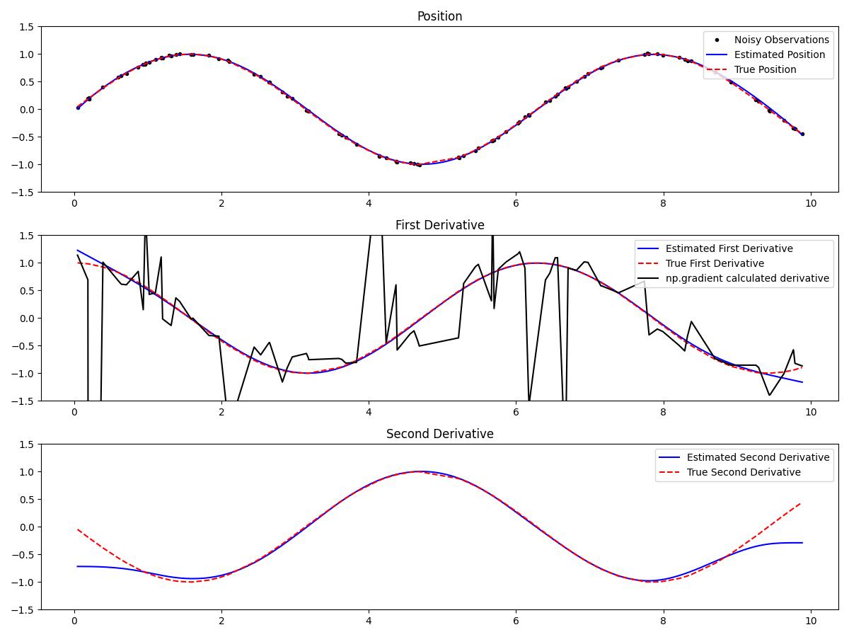
Let's walk through an example where we estimate the first and second derivatives of noisy sinusoidal data sampled at random time intervals.
import numpy as np
import matplotlib.pyplot as plt

from kalmangrad import grad  # Import the grad function

# Generate noisy sinusoidal data with random time points
np.random.seed(0)
t = sorted(np.random.uniform(0.0, 10.0, 100))
noise_std = 0.01
y = np.sin(t) + noise_std * np.random.randn(len(t))
true_first_derivative = np.cos(t)
true_second_derivative = -np.sin(t)

# Estimate derivatives using Kalmangrad
N = 2  # Order of the highest derivative to estimate
smoother_states, filter_times = grad(y, t, n=N)

# Extract estimated derivatives
estimated_position = [state.mean()[0] for state in smoother_states]
estimated_first_derivative = [state.mean()[1] for state in smoother_states]
estimated_second_derivative = [state.mean()[2] for state in smoother_states]

# Plot the results
plt.figure(figsize=(12, 9))

# Position
plt.subplot(3, 1, 1)
plt.plot(t, y, 'k.', label='Noisy Observations')
plt.plot(filter_times, estimated_position, 'b-', label='Estimated Position')
plt.plot(t, np.sin(t), 'r--', label='True Position')
plt.legend(loc='upper right')
plt.ylim(-1.5, 1.5)
plt.title('Position')

# First Derivative
plt.subplot(3, 1, 2)
plt.plot(filter_times, estimated_first_derivative, 'b-', label='Estimated First Derivative')
plt.plot(t, true_first_derivative, 'r--', label='True First Derivative')
plt.plot(
    t,
    np.gradient(y, t),
    'k-',
    label='np.gradient calculated derivative'
)
plt.legend(loc='upper right')
plt.ylim(-1.5, 1.5)
plt.title('First Derivative')

# Second Derivative
plt.subplot(3, 1, 3)
plt.plot(filter_times, estimated_second_derivative, 'b-', label='Estimated Second Derivative')
plt.plot(t, true_second_derivative, 'r--', label='True Second Derivative')
plt.legend(loc='upper right')
plt.ylim(-1.5, 1.5)
plt.title('Second Derivative')

plt.tight_layout()
plt.show()
Function Overview
The core functions in Kalmangrad are designed to be intuitive and flexible.
grad(y, t, n=1, delta_t=None, obs_noise_std=1e-2, online=False, final_cov=1e-4)
Estimates the derivatives of the input data y up to order n using Bayesian filtering and smoothing.
Parameters:
y(np.ndarray): Observed data array.t(np.ndarray): Time points corresponding toy.n(int, optional): Maximum order of derivative to estimate (default is 1).delta_t(float, optional): Time step for the Bayesian filter. If None, it's automatically determined.obs_noise_std(float, optional): Standard deviation of the observation noise (default 1e-2).online(bool, optional): If True, runs the filter in an online fashion. Default is False.final_cov(float, optional): Final covariance on the diagonal of the process noise matrix.
Returns:
smoother_states(List[Gaussian]): List of Gaussian states containing mean and covariance estimates for each derivative.filter_times(np.ndarray): Time points corresponding to the estimates.
Dependencies
Kalmangrad keeps dependencies minimal:
- Python 3.x
- NumPy: For numerical computations.
- BayesFilter: For Bayesian filtering and smoothing.
You can install the dependencies via:
pip install numpy bayesfilter
Conclusion
Kalmangrad provides a powerful and flexible tool for estimating higher-order derivatives from noisy, non-uniformly sampled data. By leveraging Bayesian filtering techniques, it offers a robust alternative to traditional numerical differentiation methods, enabling more accurate and reliable analysis in your projects.
The full code and documentation are available on GitHub. Feel free to contribute, report issues, or suggest improvements.
License
This project is licensed under the MIT License - see the LICENSE file for details.